Quick Links:
Lectures:
Last updated at 11:47 PM on 18 Mar 2007
![]() Subscribe to the
RSS feed for lecture podcasts.
Subscribe to the
RSS feed for lecture podcasts.
18. Psychometric Chart and Air-Conditioning Processes
Lecture on 15 March 2007
Reading: Cengel and Boles: 14.5 -- 14.7
Learning Objectives
- Be able to read moist air properties from a psychrometric chart.
- Be able to sketch a pure heating process and a heating with humidification process on a psychrometric chart.
- Be able to apply mass and energy balances to heating/cooling and humidifying/dehumidifying processes of moist air streams.
Announcements
The final exam is Tuesday, 20 March 2007, 10:15 AM to 12:05 PM. Bring a calculator and a two-sided cheat sheet.
Hand Notes
I didn't cover as much material as I planned to cover during lecture. Here are my handwritten notes on air-conditioning process. The notes are very similar to the material in Chapter 14.
17. Gas Mixtures and Properties of Moist Air
Lecture on 13 March 2007
Reading: Cengel and Boles: 14.1 -- 14.3
Slides: [one per page]
Learning Objectives
- Be able to define the humidity ratio: mv/ma
- Be able to compute the humidity ratio the the partial pressure of the water vapor in the air
- Be able to compute the humidity ratio from the relative humidity an temperature.
- Be able to define the relative humidity and compute it from vapor pressure data or from the humidity ratio and saturation pressure data.
Textbook Reading
Review the Steady flow energy equation: Cengel and Boles Equation (5-37), p. 231 and study the first part of Chapter 14.
16. Gas Mixtures and Properties of Moist Air
Lecture on 8 March 2007
Reading: Cengel and Boles, 13.3, 14.1 -- 14.2
Learning Objectives
- Be able to compute the (extensive) internal energy of a mixture from the internal energy per mole of the constituents.
- Be able to compute the (extensive) enthalpy of a mixture from the enthalpy per mole of the constituents.
- Be able to compute the (extensive) entropy of a mixture from the entropy per mole of the constituents.
- Be able to compute the internal energy per mole (or per unit mass) of a mixture from the internal energy per mole (or per unit mass) of the constituents.
- Be able to compute the enthalpy per mole (or per unit mass) of a mixture from the enthalpy per mole (or per unit mass) of the constituents.
- Be able to compute the entropy per mole (or per unit mass) of a mixture from the entropy per mole (or per unit mass) of the constituents.
- Be able to compute the average (molar or gravimetric) specific heats (at constant volume or constant pressure) of a mixture from the (molar or gravimetric) specific heats of the constitutents.
- Be able to qualitatively define dry air and atmospheric air in terms of its moisture content.
- Be able to quantitatively relate the pressure of atmospheric air to the partial pressure of the moisture and partial pressure of dry air in the atmospheric air sample.
- Be able to define the humidity ratio (or absolute humidity or specific humidity) for atmospheric air.
- Be able to compute the humidity ratio of atmospheric air given the partial pressure of water vapor in the air.
- Be able to define relative humidity.
- Be able to compute humidity ratio of relative humidity, and vice versa.
In-Class Worksheet
I handed out this worksheet on computing the humidity ratio given the relative humidity.
15. Gas Mixtures
Lecture on 6 March 2007
Reading: Cengel and Boles, 13.1 -- 13.2
Learning Objectives
- Be able to explain the difference between a molar basis and a gravimetric basis for intensive thermodynamic properties.
- Be able to define and compute the mass fraction and mole fraction of constituents of a mixture.
- Be able to compute the average molar mass of a mixture.
- Be able to compute the average gas constant of a gas mixture.
- Be able to use Dalton's law to compute the pressure of a mixture from the partial pressures of the constituents.
- Be able to use Amagat's law to compute the volume of a mixture from the partial volumes of the constituents.
- Be able to state the conditions required for Dalton's Law and Amagat's Law to give the same results.
- Know how to relate the partial pressure to the mole fraction and mixture pressure of a ideal gas.
- Know how to relate the partial volume to the mole fraction and mixture volume of a ideal gas.
- Be able to define the compressibility of a gas mixture.
- Be able to compute the reduced critical pressure and the reduced critical temperature of a gas mixture.
- Be able to describe how Kay's rule is used to compute the p-v-T behavior of a gas mixture.
Extra Worksheet
I did not hand out this worksheet on computing the mass fraction of the constituents of air, but you may find it helpful as you study.
Textbook Reading
Chapter 12 of the book by Cengel and Boles contains definitions that are useful in subsequent chapters. The material is not difficult, but do not be deceived. As with all definitions, these formulas must be used with precision.
14. Isentropic Property Relationships for Compressible Flow
Lecture on 1 March 2007
Reading: 11.4
Learning Objectives
- Be able to evaluate the isentropic relationships for the stagnation properties
- Be able to explain the physical significance of the * states.
Announcements
Problem Set #6 is Due on Tuesday, March 6. Do problems 11.6, 11.7, 11.32, 11.36, 11.46
Gerry will be in Salem on Monday, March 5. No office hours on Monday.
Quiz #2 will be on Tuesday, March 6. It will last 15 minutes and cover compressible flow only.
In-Class Worksheet
During class we worked on some example problems related to compressibility and ideal gas properties. You can download the sample problems and solutions distributed during lecture. Note that there is a typo in the worksheet. The supply temperature of the gas in problem 6 is 540 F, not 540 R. The version of the work sheet you can download has been corrected.
Handwritten Notes
I did a quick derivation of a formula for computing the flow rate for compressible flow through an orifice. You can download a scanned copy of those notes to fill in the details and read additional information I didn't cover in class.
13. Introduction to Compressible Flow
Lecture on 27 February 2007
Reading: 11.1 -- 11.3
Slides: [one per page]
Learning Objectives
- Be able to list fluid properties associated with compressible flow.
- Be able to use and manipulate isentropic relationships between p, T, and rho, for example, p/rhok = constant.
- Be able to write (from memory) and correctly use the formula for speed of sound of an ideal gas.
- Be able to compute the Mach number and use its value to correctly identify the flow regime.
- Be able to predict whether a compressible flow will increase or decrease as a result of area change and the current value of Ma.
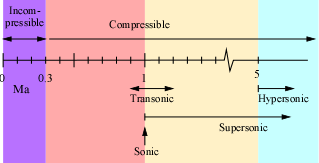
Mach Number Ranges
The general rule of thumb is that when Ma < 0.3 a gas flow can be treated as incompressible. In the compressible flow regime, any flow with Ma > 1 is said to be supersonic. Flows with Mach numbers in the range 0.9 < Ma < 1.2 are said to be transonic. Flows with Ma > 5 are said to be hypersonic. These ranges are represented graphically in the following diagram.
12. Matching Pumps and Systems, Pump Similarity
Lecture on 22 February 2007
Reading: 12.4 -- 12.5
Guess Lecture by Professor Weislogel.
11. Matching Pumps and Systems
Lecture on 20 February 2007
Reading: 12.3 -- 12.4
Slides: [one per page]
Learning Objectives
- Be able to sketch a basic system curve.
- Be able to modify a sketch of a system curve to take into account changes in elevation and changes in valve settings.
- Be able to define NPSH, NPSHA, and NPSHR
- Be able to define the vapor pressure of a liquid
- Be able to explain why maintaining adequate NPSH is necessary for pump operation.
- Be able to sketch the balance point of a system and a pump.
- Be able to show how the balance point changes when a valve in the system changes.
- Be able to identify the role of pump efficiency and motor efficiency in overall system performance.
Announcements
Guest lecture by Professor Weislogel next Thursday. Regular course topics (end of pumps, beginning of compressible flow) and maybe some extra goodies.
Career Fair at the Career Center
PSU Career Fair on February 28 at SMU Ballroom. http://www.pdx.edu/careers/careerfairs.html
Podcast
Part B of the podcast (for the second half of class) just ends. I must have hit the stop button by accident when the recorder was in my pocket.
Gear Pumps
During the last class (Lecture #10) we had a discussion about how gear pumps work. I gave myself the assignment to get more information. I found these web pages with gear pump animations
- RPI Chemical Engineering Page
- A student report from MIT
- Gear animations at drgear.com
- Allstar Network at Florida International University
Lecture Notes
A Simple pump model was presented
-
Identify velocity components U, V, W
V = absolute velocity of the fluid
- Velocity triangles
- Use angular momentum conservation to get simple formula for Torque and Fluid Power
- Simple model of head versus flow rate for the case of zero inlet swirl
Detailed handwritten notes on the pump model can be downloaded here
CFD in Pump Design
Computational Fluid Dynamics or CFD is the use of numerical models to predict fluid flow. Centrifugal pumps have complicated geometries that can be analyzed with CFD. Here is a sample article on using CFD for water pump design
10. Overview of Turbomachinery
Lecture on 15 February 2007
Reading: 12.1 -- 12.4
Slides: [one per page]
Learning Objectives
- Be able to describe the key differences between positive displacement pumps and dynamic pumps (turbomachines).
- Be able to describe the key features of a pump curve: what are maximum flow and maximum head conditions?
- Be able to create a pump curve, h = f(Q), when given data from a pump test stand.
Announcements
Career Fair at the Career Center
PSU Career Fair on February 28 at SMU Ballroom. http://www.pdx.edu/careers/careerfairs.html
Example from Fox and MacDonald
We worked on a sample problem involving the conversion of measured pump data to a pump curve.
- Problem statement (PDF)
- Data in m-file (MATLAB)
- Completed Solution (MATLAB)
9. Separation, Empirical Data for Drag
Lecture on 8 February 2007
Reading: 9.3
Slides: [one per page]
Learning Objectives
- Be able to apply the Bernoulli equation to a streamline outside the boundary layer and derive the relationship between pressure gradient and variation in free stream flow.
- Be able qualitatively describe the relationship between changes in the free stream velocity and the pressure gradient
- Be able to qualitatively describe the difference between form drag and skin friction.
- Be able to write the definition of the drag coefficient.
- Be able to define and compute the frontal area of simple geometric objects.
- Be able to compute the drag force on an object given its dimensions, the free stream velocity, and a drag coefficient.
- Be able to look up drag coefficients from tables in the textbook.
Announcements
The midterm exam is Tuesday, 13 February 2007.
- The exam is comprehensive: it covers everything up to and including today's lecture.
- The exam will take the entire class period -- don't be late!
- You are allowed a cheat sheet constructed from a single sheet of 8.5 x 11 inch paper. You are allowed to write on only one side of the cheat sheet.
- Test questions will include both short-answer type questions and longer problems.
- A universal cheat sheet will be provided with the exam.
- A Moody chart will be provided. It's possible that tabular data will be provided.
- Bring your calculator.
Video Segments
- 9.4 CFD Simulation and Snow Drifts
- 9.5 Sky Diving Practice: Drag during Freefall
- 9.7 Boundary Layers and Wakes for a Jet Ski
- 9.8 Flow around a truck
8. Turbulent Boundary Layers, Separation
Lecture on 6 February 2007
Reading: 9.2
Learning Objectives
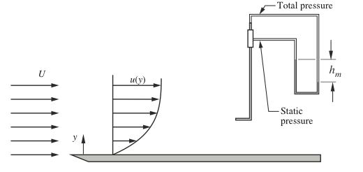
- Be able apply the definitions of delta, delta99, delta* when given data or a formula for u(y)
- Be able to use appropriate formulas for computing the shear stress on a flat plate aligned with the flow. Both turbulent and laminar flow.
Announcements
Quiz 1 is graded. The solution is available on the web page for exams.
The midterm exam is Tuesday, 12 February 2007. It covers everything up to and including next Thursday's lecture (through lecture 9).
Solution to Problem 9.13 in the Textbook
- Typeset solution to Exercise 9.13.
- Schematic
- Data Table
- MATLAB code containing data only
- Complete solution in MATLAB
7. Analysis of Flat Plate Boundary Layers
Lecture on 1 February 2007
Reading: 9.1 -- 9.2
Podcast: [Part A] [Part B] [Part C]
Slides: [one per page]
Learning Objectives
- Be able to give verbal and mathematical definitions for three measures of boundary layer thickness: the physical "delta-99", the displacement thickness, and the momentum thickness.
- Be able to discuss the meaning of "thin" for a boundary layer, especially as it relates to the results of scale analysis.
- Be able to apply formulas for boundary layer thickness and drag for a laminar boundary layer.
- Memorize the critical Reynolds number for transition to turbulence for a flat plate boundary layer.
Announcements
Quiz 1 is not graded. I'll create a web page for exams and solutions.
In-Class Exercise
In the second half of class we began the solution to this in-class worksheet.
Historical Figures in Aerodynamics
Here are Wikipedia links to Ludwig Prandtl and Theodore von Karman.
John Anderson wrote an article giving a historical account of Prandtl's boundary layer theory. Anderson has also written a textbook on the History of Aerodynamics. [Amazon Link] [Book Review from ASEE Prism]
Textbook Reading
The book refers to the boundary layer thickness as "delta" for what I called "delta99". The "delta99" designation is somewhat more common in the boundary layer literature.
6. Obstruction Flow Meters; Introduction to External Flow
Lecture on 30 January 2007
Reading: 8.6, 9.1
Slides: [one per page]
Learning Objectives
- Be able to compute the flow rate through orifice meters, long radius nozzles and Venturi flow meters given meter dimensions and the pressure drop.
- Be able to define the Reynolds number (i.e. specify the appropriate length scale and velocity scale) for flow past a flat plate.
- Be able to list the qualitative features of a boundary layer.
- Be able to make distinction between drag and lift forces
- Be able to explain why streamlines adjacent to a flat plate are angled away from the plate.
Announcements
The bookstore now has Thermodynamics books in stock. The fifth edition (the one sold last quarter) is no longer available. The bookstore has the sixth edition of Thermodynamics: an Engineering Approach, by Cengel and Boles. You do not need to buy the new edition. However, if you don't yet have a copy of the book, and if you want to get a copy, you can buy the latest edition at the PSU Bookstore.
Introduction to External Flow
In an external flow the object of interest is immersed in a fluid with large extent. Examples include
- the wing of an aircraft moving through a stationary fluid
- a ball flying through the air
- structures protruding into a flow: buildings, trees, support beams flow probes
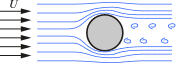
Boundary layers exist when there are high velocity and/or large length scales: viscous effects are confined to a thin layer near the wall.
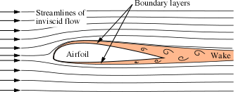
Caution: Not all external flows are fully explained by boundary layers. Boundary layer analysis is especially useful for streamlined objects, i.e. objects that do not cause large disruption in the streamlines of the on-coming flow. A "large disruption" occurs when the object causes the streamlines to displace by an amount equal to the size of the object.
Goals
- Develop basic awareness of boundary layer concepts
- Understand flow physics that affect drag on external objects
- Understand basic features of boundary layer velocity profile
Engineering Applications
- Calculating drag
- Predicting thickness of boundary layers
5. Non-Circular Pipes; Three Types of Pipe Flow Problems; Series and Parallel Pipes
Lecture on 25 January 2007
Reading: 8.4.3 -- 8.5
Podcast link
Slides: [one per page]
Learning Objectives
- Be able to apply head loss calculations to ducts with non-circular cross sections.
- Be able to name the three basic types of pipe flow problems.
- Be able to recognize and set up the analysis for three basic types of pipe flow problems.
- Be able to state the basic rules governing head loss and flow rate for two pipes in parallel.
- Be able to state the basic rules governing head loss and flow rate for two pipes in series.
In-Class Exercise
For practice, we worked on this example problem.
MATLAB Toolbox
In class I mentioned a MATLAB Toolbox for analyzing pipe flow. I've been working on the documentation for the Toolbox and you can download an alpha version of the documentation and you can download a ZIP archive of the MATLAB programs. The class is not expected to use this toolbox and the programs. Adventurous students are encouraged to play with this code. Recognize that the documentation is "alpha" quality, meaning that it is incomplete and possibly contains errors.
4. Viscous Head Loss in Round Pipes
Lecture on 23 January 2007
Reading: 8.4.1 -- 8.4.2
Podcast link
Slides: [one per page]
Learning Objectives
- Be able to use the Energy Equation, Darcy-Weisbach Equation, and the Colebrook Equation (or Moody chart) to compute head loss in a long straight section of pipe. (A.k.a. "major loss")
- Be able to use reference charts, tables, formulas to obtain minor loss coefficients.
- Be able to combine major and minor losses to predict head loss in a continuous pipe. (A pipe with a single passageway.)
Sample Calculations
We worked the solution to problems 1 and 2 on this worksheet. You should also be able to do problems 3 and 4 on your own.
Solving the Colebrook Equation with MATLAB
I demonstrated how to use the moody.m
function to solve the Colebrook equation with MATLAB. The steps are
-
Download
moody.m(Right-click and "Save As ...") - Launch MATLAB
-
Navigate (inside MATLAB) to the directory that contains
moody.m -
Assign values to
ReDandeDand then typef = moody(eD,ReD)
Here's a sample session
   >> ReD = 5.5e6;   eD=0.003;
   >> f = moody(eD,ReD)
   f =
       0.0262
3. Introduction, Differential Analysis of Fluid Flow
Lecture on 18 January 2007
Reading: 8.2 - 8.4
Podcast link
Slides: [one per page]
Learning Objectives
- Be able to solve the ODE for the laminar velocity profile in a round tube, and extract all meaningful engineering quantities from the solution
- Be able to work with formulas fully developed laminar flow in a pipe: u(r), Vc, and Q as function of pressure gradient
- Be able to write the formula for the friction factor for fully developed laminar flow in a round pipe.
- Be able to identify the major regions of the Moody chart.
- Be able to use the Moody chart to obtain the friction factor given the Reynolds number and the relative roughness of the pipe.
Announcements
There was no class on Tuesday, 16 January. I'll try to make up a little time, but I can't forsee omitting an entire class worth of material from this part of the course.
Problem set 2 is available from the homework page.
Notes
I mentioned that a root-finding procedure can be used to find the friction factor from the Colebrook equation. The moody.m file is a MATLAB function for finding f when Re and epsilon/D are given.
Textbook Reading
I followed the text in section 8.2 quite closely except that I skipped section 8.2.2.
I went rather quickly over the material in sections 8.3.1 through 8.3.3. Please read those sections, but try not to get bogged down in the terminology. I skipped the material in section 8.3.4 and 8.3.5. Those sections interesting, but not essential for a first course in applied fluid mechanics.
Section 8.4 is very important for practical applications. We only covered section 8.4.1 in class today.
2. Overview of Internal Viscous Flow
Lecture on 11 January 2007
Reading: 8.1 - 8.2
Learning Objectives
- Be able to recognize whether flow of liquid in an conduit is considered pipe flow or open channel flow
- Be able to identify/name the general characteristics of turbulent flow
- Be able to define and quantitatively estimate the entrance length for laminar and turbulent flow.
- Be able to identify/name the general characterisics of fully-developed flow.
Movies
To motivate a physical understanding of turbulence I showed three movie clips from textbook multimedia resources.
8.1: Laminar/Turbulent Pipe flow
This clip shows a modern interpretation of the famous experiment by Reynolds. The frame shows water flowing through a transparent, horizontal pipe. Dye is injected into the center of the pipe.
As the clip progresses, the velocity of the water through the pipe is increased. At very low water velocity the filament of dye-colored water is straight. As the velocity is increased, the dye streak becomes unsteady. At low speeds the dye streak is wavy or "sinuous" to use Reynolds' term. Increasing the speed further causes the dye streak to become very disordered. At the highest speeds the turbulence in the pipe causes the dye to become so well mixed that it is only visible as a slightly darker color that spans almost the entire cross section of the pipe.
From this video we conclude that turbulence is unsteady and appears to be random or chaotic. The turbulent flow has significant cross-stream velocity components which cause any convected quantity (the dye in the video clip) in the flow to be well mixed.
8.2: Turbulence in a bowl
The video clip shows a shallow bowl of liquid being stirred by a spoon. The liquid has suspended metal flakes that make it possible to see the currents. The metal flakes change orientation, and hence reflectivity, as they move with the fluid. Although stirring the liquid in the bowl causes waves on the surface, the fine details of the flow structure is not due to waviness of the surface.
The detailed flow structure revealed by the metal flakes reveals that (1) turbulence involves motion at many length scales, (2) when the stirring stops, energy is no longer added to the system and the motion decays, and (3) the small scale motions are dissipated first, which causes the flow structure to appear more smooth as time progresses after stirring stops.
8.3: Laminar/turbulent velocity profiles
This clip shows laminar and turbulent velocity profiles in a pipe. The video frame is a view of a small length of the vertically oriented pipe. Out of the frame and below the test section is a valve that is used to start the flow. Initially the fluid is stationary. After a brief preparation sequence, the valve is opened and the velocity profile is made visible by the motion of a dye streak that starts out as a horizontal line near the top of the video frame.
At the beginning of each demonstration, a needle filled with dye is slowly withdrawn from the pipe. The needle moves horizontally from right to left. As the needle is withdrawn from the pipe, dye is injected into the stationary fluid. After the needle has been completely removed from the pipe, the valve is opened, thereby allowing the fluid to flow downward through the test section.
Two experiments are performed: one with a viscous oil and the other with water. The oil has a sufficiently high viscosity that its flow is laminar. In the bottom of the video frame is a label indicating that the Reynolds number is approximately equal to 1. The no-slip condition is clearly visible at the pipe walls. The velocity profile looks like a parabola.
The water has a low enough viscosity that when the valve is opened the flow is turbulent. Technically the flow will take time to become "fully" turbulent, but the steep gradient at the wall, the nearly flat average velocity profile in the center of the pipe, and the smearing of the dye in the center of the pipe are all characteristic of turbulent flow.
Textbook Reading
To do the homework you will need to read pp. 401 through 406. At the end of class I began a discussion of developing and fully-developed flow. Equation (8.1) and Equation (8.2) allow prediction of length of pipe necessary for the flow to become fully-developed.
1. Introduction, Differential Analysis of Fluid Flow
Lecture on 9 January 2007
Reading: 6.1 - 6.3
Learning Objectives
- Be able to write the substantial derivative in vector form.
- Be able to write down the differential form of the continuity equation in Cartesian coordinates and in vector form.
- Be able to Evaluate a formula for the velocity field to determine whether it satisfies the continuity equation.
- Be able to show that the stream function for incompressible two-dimensional flow automatically satisfies the continuity equation.
- Recognize that for two dimensional, incompressible flow, streamlines are lines of constant stream function
- Be able to indentify the main terms in the Cauchy equations of motion -- Equations (6.50)
Handouts (PDF)
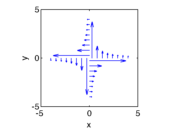
Example Problem: Velocity field for a Free Vortex
I had the class work through a
problem to verify whether a vector field satisfied the
continuity equation for two-dimensional incompressible flow.
The image below shows one representation of the free vector created by
vortexVectors MATLAB function.
Textbook Reading
Chapter 5 deals with finite control volumes: macroscopic scale regions of space. With finite control volumes, we use data on the velocity entering and leaving the control volume and the net forces acting on the control volume. Overall balances of mass, momentum and energy on the control volume do not give us detailed information on what happens inside the control volume.
Chapter 6 provides an overview to differential analysis of fluid motion. Differential analysis provides a framework for predicting the velocity field, i.e. the velocity at each point in space inside a domain of interest. In principle, differential analysis gives us much more detail than finite control volume analysis. However, the detail requires more sophisticated mathematical analysis.
In fact, very few flows can be analyzed by purely mathematical means: the equations are just too difficult to solve. Historically this meant that only highly simplified flows could be analysized using differential analysis. Now, we have numerical techniques -- usually called Computational Fluid Dynamics or CFD -- to obtain approximate solutions to the differential equations. Appendix A provides a brief introduction to CFD.
In ME 322 we will study only part of Chapter 6. The overall goal is to gain an awareness of differential analysis. Students interested in more advanced study of fluid mechanics will need to take additional courses, e.g. ME 441, to learn about differential analysis.
Although we will only be studying sections 6.1 - 6.3 and 6.8, it is helpful to get an overall picture of the chapter.
- Sections 6.1-6.3 provide a very quick development of a general form of the equations of motion (Mass and Momentum conservation) for fluids. The equations of motion are a coupled set of nonlinear partial differential equations (PDEs). These equations are quite general and difficult to work with. Numerical solutions are becoming more common, but still require advanced training.
- Sections 6.4 - 6.7 present mathematical models of flow having negligible dependence on fluid viscosity. Although viscous effects are almost always present, it is possible to learn a lot about a large class of flows by neglecting viscosity altogether. In particular, inviscid flow modeling is very useful for analzing the flow of air past aircraft. We will skip this subject entirely, but there's a chance that the models in section 6.4 - 6.7 might be useful to you in your future engineering careers. Note that section 6.4 involves a derivation of the Bernoulli equation from the differential equations of motion.
- Section 6.8 is a very quick summary of how the constitutive law for Newtonian fluids is introduced into the equations of motion presented in section 6.3. The result is the Navier-Stokes equations: the equations of motin for Newtonian fluids.
- Section 6.9 presents some of the more simple solutions to the Navier-Stokes equations. The flow models in section 6.9 are very important, but we will not dwell on them. You should be aware that these solutions exist and that you will consult a textbook (such as Munson, Young and Okiishi) when you need details of the velocity field for simple flows of Newtonian fluids.