Introduction to the MATLAB PDE codes

Table of contents

1. Overview
2. Practice with MATLAB PDE tools
   1. Launch MATLAB
   2. Working with the input and output arguments of the demoBTCS code
   3. Demonstrate convergence of demoBTCS

Overview

This page demonstrates some basic MATLAB features of the finite-difference codes for the one-dimensional heat equation. This is a MATLAB tutorial without much interpretation of the PDE solution itself. Consult another web page for links to documentation on the finite-difference solution to the heat equation.

This page is part of a series of MATLAB tutorials for ME 448/548:

Practice with MATLAB PDE tools

While we’re practicing with MATLAB, we will preview some of the codes we’ll use in the coming weeks. The goal is to get used to running the codes and storing results

The following tutorial assumes that you have configured MATLAB according to our recommendations. If not, MATLAB will not be able to find the codes.

Launch MATLAB

Launch MATLAB and move to a working directory, e.g. practice or homework. Create that directory if you haven’t already, and add it to the MATLAB path

Working with the input and output arguments of the demoBTCS code

The demoBTCS code solves the one-dimensional heat equation on $0\le x\le L$ with boundary conditions of zero at $x=0$ and $x=L$. The initial condition is a half sine wave, $u_0= sin(\pi x/L)$.

To see how to use demoBTCS, type help demoBTCS at the command prompt

>> help demoBTCS

  demoBTCS  Solve 1D heat equation with BTCS scheme on a uniform mesh
 
  Synopsis:  demoBTCS
             demoBTCS(nx)
             demoBTCS(nx,nt)
             err = demoBTCS(...)
 
  Input:  nx = number of x-direction nodes  Default:  nx = 11
          nt = number of time steps         Default:  nt = 50
 
  Output:  err = (optional) error in the numerical solution

The Synopsis section of the help message describes four ways of calling demoBTCS. nx and nt are optional input arguments with default values of 11 and 15 respectfully

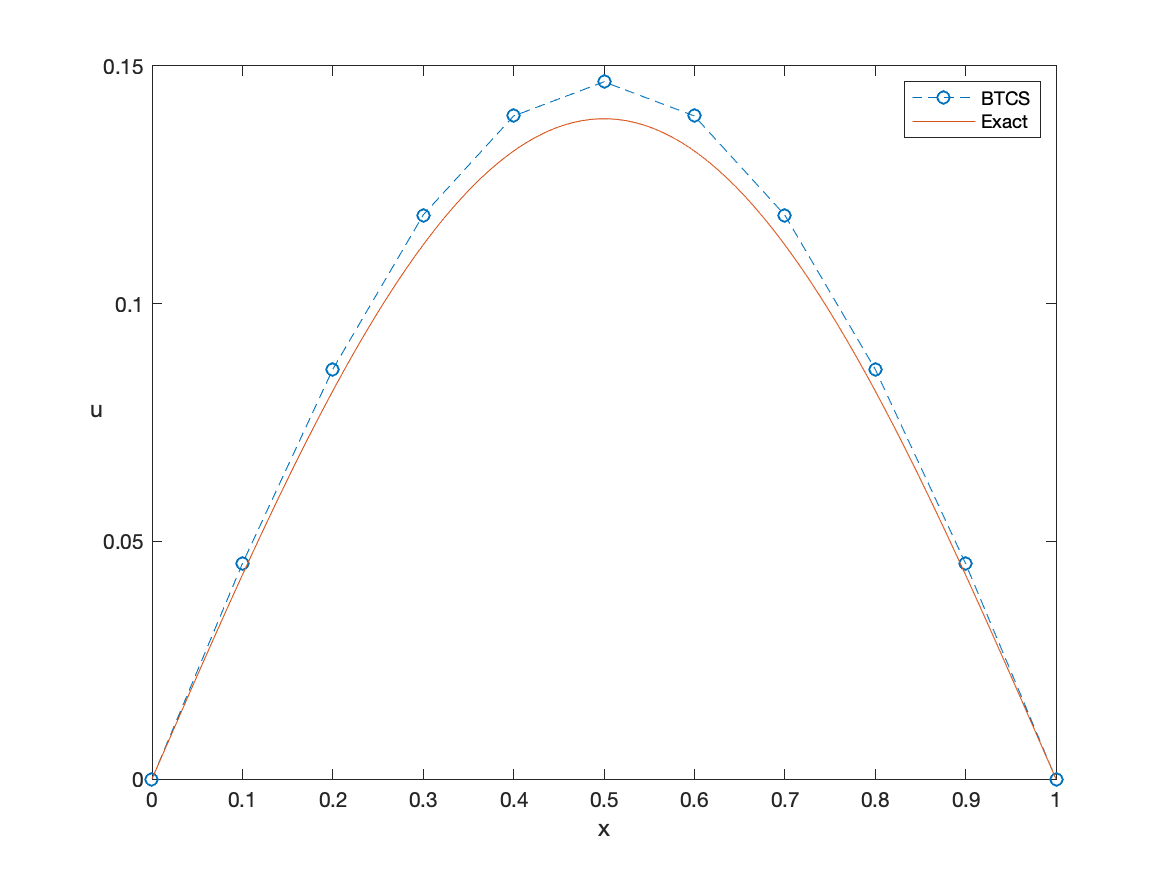
Running the demoBTCS code without any inputs produces a print out of the measured truncation error and a plot comparing the BTCS solution with the exact solution

>> demoBTCS
Error in BTCS solution = 0.005224

Demonstrate convergence of demoBTCS

As homework you will be asked to plot the truncation error of finite difference schemes as a function of mesh size. For example, we know that the error in the BTCS scheme should vary as $(\Delta x)^2 + \Delta t$. The demoFTCS, demoBTCS and demoCN schemes all have optional return arguments that give the measured error in solving the heat equation.

To create a plot of the truncation error you will need to run the code for many combinations of spatial meshes and time steps, store the measured error values for each combination, and then plot the error versus a measure of the mesh size. You could do that work manually. I recommend instead that you write a program.

Here is the first version of the program that runs the program on a series of mesh and time step combinations, and prints the results

function convergence_test

alfa = 0.1;  L = 1;  tmax=2;   rsafe = 0.49999;  %  stable r<0.5

% --- Specify nx and compute nt consistent with stability limit
nx = [8 16 32 64 128];
nt = ceil( 1 + alfa*tmax*((nx-1).^2)/(rsafe*L^2) );

% --- Loop over mesh sizes and store the error
fprintf('\n    nx     nt     error\n');
for j=1:length(nx)
  err = demoBTCS(nx(j),nt(j));
  fprintf(' %5d  %5d  %11.3e\n',nx(j),nt(j),err);
end

end

Notice that the output of the demoBTCS function is stored in a variable called err. That allows the value of err to be printed in a nice tabular format.

Also notice that the progression of x-direction mesh sizes is in powers of 2, not multipoes of 2. To see the trend in mesh refinement, large changes in mesh size are generally necessary.

Finally, notice that the number of time steps, nt is also increased rapidly with nx. We will dig into that in a later lecture.

Running convergence_test produces the following text output

>> convergence_test
>> close all; convergence_test

    nx     nt     error
     8     21    6.028e-03
    16     92    1.356e-03
    32    386    3.262e-04
    64   1589    7.972e-05
   128   6453    1.970e-05

To plot the truncation error as function of mesh size we need to store the truncation error values in a vector. It would also be good to compute $\Delta x$ values.

Add the following lines to create the dx and err vectors

dx = L./(nx-1);

err = zeros(length(nx),1);

Change these lines involving err

  err(j) = demoBTCS(nx(j),nt(j));
  fprintf(' %5d  %5d  %11.3e\n',nx(j),nt(j),err(j));

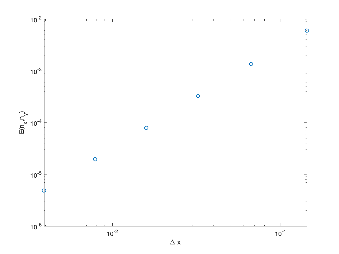
Now that dx and err vectors are available after the for loop is complete, add the following lines to create the plot of truncation error versus $\Delta x$

loglog(dx,err,'o');
xlabel('\Delta x');   ylabel('E(n_x,n_y)');

The completed function, with comment statements, is

function convergence_test
% convergence_test  Plot truncation error of BTCS versus delta x

alfa = 0.1;  L = 1;  tmax=2;   rsafe = 0.49999;  %  stable r<0.5

% --- Specify nx and compute nt consistent with stability limit
nx = [8 16 32 64 128 256];
dx = L./(nx-1);
nt = ceil( 1 + alfa*tmax*((nx-1).^2)/(rsafe*L^2) );
err = zeros(length(nx),1);

% --- Loop over mesh sizes and store the error
fprintf('\n    nx     nt     error\n');
for j=1:length(nx)
  err(j) = demoBTCS(nx(j),nt(j));
  fprintf(' %5d  %5d  %11.3e\n',nx(j),nt(j),err(j));
end

% --- Plot measured error
loglog(dx,err,'o');
xlabel('\Delta x');   ylabel('E(n_x,n_y)');

end

Running this modified version of convergence_test produces the following plot

To see how the choice of nt affects the result, comment out the existing definition of nt and replace it with a vector of constant values

% nt = ceil( 1 + alfa*tmax*((nx-1).^2)/(rsafe*L^2) );
nt = 512*ones(size(nx));

and rerun the convergence_test code. How is this result (with constant nt) different from the results with nt increasing in proportion to the square of nx?