A Recipe for Finding Multiple Roots of $f(x)=0$

A preceding recipe shows how to find a single root of $f(x)=0$ with the brackPlot and bisect functions. This example shows how the procedure for finding a single root can be extended to the case where $f(x)$ has multiple roots in the region of interest. The goal is to find all of the roots in an automated way.

In this example, I walk you through the following steps

1. Identify good bracket intervals that contain roots.
2. Use bisection to refine the guess at the roots within each of the bracketing interval.
3. Separate the roots from the singularities.

The case of multiple roots requires some modification to the simpler, single-root example. Step 2 involves a loop over each of the brackets. Step 3 requires distinguishing the roots and singularities for multiple different potential roots.

Although the code logic is a little more complicated for multiple roots, the final solution is obtained with a relatively brief, and ultimately straightforward MATLAB code.

The Example Problem

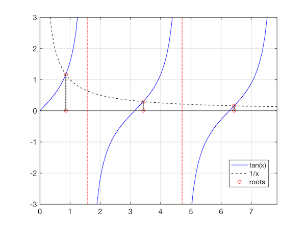
We demonstrate the technique for finding multiple roots by finding the values of $x$ that satisfy

or

To make the example problem more interesting, we will find all 8 roots on the interval $-4\pi\le x\le 4\pi$.

A plot of $y=\mathrm{tan}(x)$ and $y=1/x$ shows that those curves intersect at multiple points. For example, the following plot shows the first three roots for $x>0$. The roots are identified as open circles at the points where $y=\mathrm{tan}(x)$ and $y=1/x$ intersect. The plot also shows the projection of those points down to the $x$ axis. Vertical dash-dot red lines indicate the singularities of the $\mathrm{tan}(x)$ function. As we shall see, the bracketing and root-finding algorithms cannot distinguish roots from singularities. We need to follow the root-finding step with a testing and sorting step where the roots and singularities are separated.

1. Find Bracket Intervals for $f(x)=0$

As with the single-root example, we begin by writing a small m-file that evaluates $f(x)$. The following code is stored in the tan1x.m file.

function z = tan1x(x)
z = tan(x) - 1./x;
end

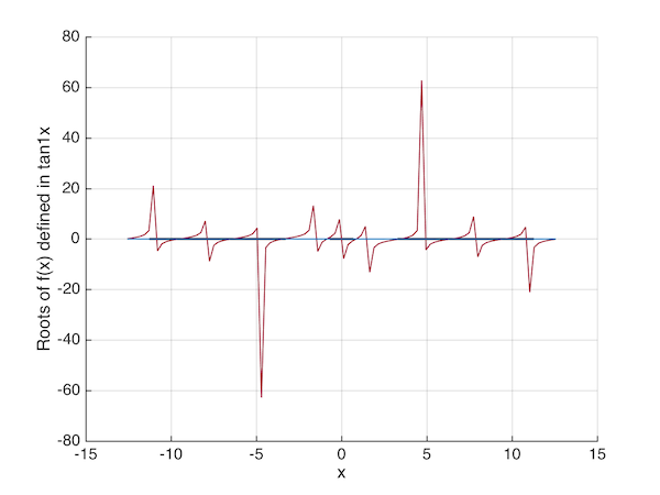
Running the brackPlot helper function on the interval $-4\pi\le x\le 4\pi$ produces the following text output and plot

>> xb = brackPlot('tan1x', -4*pi, 4*pi)
xb =
  -11.2436   -9.9208
   -9.9208   -8.5980
   -8.5980   -7.2753
   -7.2753   -5.9525
   -5.9525   -4.6297
   -4.6297   -3.3069
   -0.6614    0.6614
    3.3069    4.6297
    4.6297    5.9525
    5.9525    7.2753
    7.2753    8.5980
    8.5980    9.9208
    9.9208   11.2436

The brackets returned by brackPlot are stored in xb, which has 13 rows.

>> nb = size(xb,1)
nb =
    13

The plot is not particularly helpful because the scale of the $y$-axis is large. We can rescale the $y$ axis with the ylim command to reduce the distorting effect of the singularities of $f(x)$.

>> ylim( [-3, 3] )

Running ylim produces the following plot. (Note, we are not creating a new plot. We're just changing the $y$-axis scale on the existing plot.)

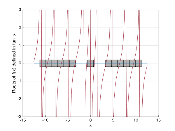
The boxes drawn by brackPlot appear to miss some of the places where $f(x)$ crosses the $x$ axis. Remember that brackPlot cannot distinguish singularities from roots, so some of the brackets identified by brackPlot contain singularities. We don't worry about that now. The immediate need is to adjust the inputs to brackPlot so that it identifies intervals for all of the roots and all of the singularities. We will distinguish the roots from the singularities after each bracket is refined by bisect.

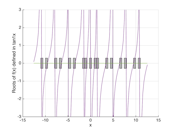
In order to force brackPlot to find brackets for all of the roots (and singularities), we use the fourth and optional input nx. For $f(x)=\mathrm{tan}(x) - 1/x$, using nx = 75 captures all of the roots on the interval $-4\pi\le x\le 4\pi$. A different $f(x)$ may require a different value of nx. A different $x$ interval for the same $f(x)$ may require a different value of nx.

Running brackPlot with 75 search intervals gives

>> xb = brackPlot('tan1x', -4*pi, 4*pi, 75)
xb =
  -11.2078  -10.8682
   -9.8493   -9.5097
   -8.1512   -7.8115
   -6.4530   -6.1134
   -4.7548   -4.4152
   -3.7359   -3.3963
   -1.6982   -1.3585
   -1.0189   -0.6793
   -0.3396         0
    0.6793    1.0189
    1.3585    1.6982
    3.3963    3.7359
    4.4152    4.7548
    6.1134    6.4530
    7.8115    8.1512
    9.5097    9.8493
   10.8682   11.2078

which is a total of 17 suspected roots

>> nb = size(xb,1)
nb =
    17

The plot produced by brackPlot with $\mathtt{nx}=75$ confirms that no roots appear to be missed.

2. Refine the Guess for Each Suspected Root

Given a list of intervals from brackPlot that contain suspected roots, we use bisect to find the roots in each interval. Since there is more than one bracket, a loop is required. Furthermore, since it awkward to write loops in the command window, we start building an m-file that implements a solution. This m-file is extended in stages throughout this example. The code is tested at each stage. By the end, we have created a single main m-file that does all of the work.

We start with tan1xRoots1, which encapsulates the commands used so far to find the brackets of suspected roots.

function tan1xRoots1(xmin,xmax,nxSearch)

if nargin<1, xmin=-4*pi;  end
if nargin<2, xmax=4*pi;   end
if nargin<3, nxSearch=75; end

% -- Use brackPlot to identify intervals that may contain roots
xb = brackPlot('tan1x',xmin,xmax,nxSearch);
ymax = 3;
ylim([-ymax, ymax])  %  Set y-axis limits to clip singularities
nb = size(xb,1);
fprintf('%d brackets found on %6.2f <= x <= %6.2f\n',nb,xmin,xmax)

end

tan1xRoots1 has input arguments xmin and xmax that allow us to change the interval over which the roots are sought. It has an input nxSearch that specifies the number of slices on $\mathtt{xmin}\le x\le \mathtt{xmax}$ that are used to search for brackets containing suspected roots.

We now add a loop over the brackets, and store the potential roots in a vector called r. The new code is called tan1xRoots2.

function tan1xRoots2(xmin,xmax,nxSearch)

if nargin<1, xmin=-4*pi;  end
if nargin<2, xmax=4*pi;   end
if nargin<3, nxSearch=75; end

xb = brackPlot('tan1x',xmin,xmax,nxSearch);
ymax = 3;
ylim([-ymax, ymax])  %  Set y-axis limits to clip singularities
nb = size(xb,1);
fprintf('%d brackets found on %6.2f <= x <= %6.2f\n',nb,xmin,xmax)

% -- Loop over the brackets
for i=1:nb
  r = bisect('tan1x',xb(i,:));
  fprintf('%4d  %8.4f\n',i,r);
end
  
end

Running the tan1xRoots2 function produces a lot of warning messages

>> tan1xRoots2
17 brackets found on -12.57 <= x <=  12.57
Warning: root not within tolerance after 50 iterations
 
> In bisect (line 53)
  In tan1xRoots1 (line 15) 
   1  -10.9956
Warning: root not within tolerance after 50 iterations
 
> In bisect (line 53)
  In tan1xRoots1 (line 15) 
   2   -9.5293
...

The warning messages indicate that the bisection algorithm has not converged to within the default tolerances after $\mathtt{maxit}=50$ iterations. Reading the bisect code, or running "help bisect" in the command window shows that xtol and ftol are optional inputs, and that their default values are both 5*eps.

>> help bisect
  bisect  Use bisection to find a root of the scalar equation f(x) = 0
 
  Synopsis:  r = bisect(fun,xb)
             r = bisect(fun,xb,xtol)
             r = bisect(fun,xb,xtol,ftol)
             r = bisect(fun,xb,xtol,ftol,verbose)
 
  Input: fun     = (string) name of function for which roots are sought
         xb      = vector of bracket endpoints. xleft = xb(1), xright = xb(2)
         xtol    = (optional) relative x tolerance.    Default:  xtol=5*eps
         ftol    = (optional) relative f(x) tolerance. Default:  ftol=5*eps
         verbose = (optional) print switch. Default: verbose=0, no printing
 
  Output:  r = root (or singularity) of the function in xb(1) <= x <= xb(2)

eps is a built-in variable with a value of $2.22\times10^{-16}$. Therefore, the default values of xtol and ftol are very small, $\sim 10^{-15}$.

>> eps
ans =
   2.2204e-16
>> 5*eps
ans =
   1.1102e-15

At this point, we have two options, either increase the values of xtol and ftol by supplying alternative values as inputs to bisect, or re-write bisect to increase the maximum number of allowed iterations, maxit. We will take the first route. Rather than rewriting bisect we relax the convergence tolerance slightly. A better, long-term solution is to use the built-in fzero function which converges much more quickly than bisect.

With some experimentation, we find that $\mathtt{xtol}=\mathtt{ftol}=5\times10^{-12}$ suppresses the warning message (by relaxing the convergence criteria) while giving a fairly tight tolerance on the roots. The tan1xRoots3 code allows the user to specify a common (xtol and ftol) tolerance with an optional input, tol. The default value of tol is $5\times10^{-12}$.

function tan1xRoots3(xmin,xmax,nxSearch,tol)

if nargin<1, xmin=-4*pi;  end
if nargin<2, xmax=4*pi;   end
if nargin<3, nxSearch=75; end
if nargin<4, tol=5.0e-12; end

% -- Use brackPlot to identify intervals that may contain roots
xb = brackPlot('tan1x',xmin,xmax,nxSearch);
ymax = 3;
ylim([-ymax, ymax])  %  Set y-axis limits to clip singularities
nb = size(xb,1);
fprintf('%d brackets found on %6.2f <= x <= %6.2f\n',nb,xmin,xmax)

% -- Loop over the brackets.  Store each root temporarily in r
for i=1:nb
  r = bisect('tan1x',xb(i,:),tol,tol);
  fprintf('%4d  %8.4f\n',i,r);
end

end

When we run tan1xRoots3 there are no warning messages and we get a list of potential roots. However, we know that brackPlot captures singularities as well as roots, so the next step is to isolate the roots from the singularities.

3. Isolating the True Roots

From our initial plot, and from our knowledge of the behavior of $\mathrm{tan}(x)$ and $1/x$, we know that $f(x)=\mathrm{tan}(x)-1/x$ has roots as well as singularities on $-4\pi\le x\le 4\pi$.

To identify the singularities we test the value of $f(r)$ for every potential root, $r$, returned by bisect. After some experimentation, a threshold of $5\times10^{-9}$ on $f(r)$ was found to correctly determine whether $r$ was a true root. In other words, when $|f(r)|<5\times10^{-9}$, we assume that $r$ is a true root, otherwise we assume that $r$ is a singularity. The tan1xRoots4 prints $r$ and $f(r)$ for every suspected root and prints "singularity!" on the same line as any r values that does not appear to be a true root.

function tan1xRoots4(xmin,xmax,nxSearch,tol)

if nargin<1, xmin=-4*pi;  end
if nargin<2, xmax=4*pi;   end
if nargin<3, nxSearch=75; end
if nargin<4, tol=5.0e-12; end

% -- Use brackPlot to identify intervals that may contain roots
xb = brackPlot('tan1x',xmin,xmax,nxSearch);
ymax = 3;
ylim([-ymax, ymax])  %  Set y-axis limits to clip singularities
nb = size(xb,1);
fprintf('%d brackets found on %6.2f <= x <= %6.2f\n',nb,xmin,xmax)

% -- Loop over the brackets.  Store each root temporarily in r
fprintf('\n   i     r           f(r)\n')
for i=1:nb
  
  % -- Refine the bracket to isolate the root or singularity
  r = bisect('tan1x',xb(i,:),tol,tol);

  % -- Print the suspected root, and the value of f(x) there
  fr = tan1x(r);
  fprintf('%4d  %8.4f  %12.3e',i,r,fr);
  
  % -- Test the magnitude of f(r) to identify true roots
  %    Assume that abs(fr)<5e-9 for a true root
  if abs(fr)<5.0e-9
    fprintf('\n')     %  End the line if we have true root
  else
    fprintf('  Singularity!\n')  %  Print message and end the line
  end
end

end

Running tan1xRoots4 produces the following output

>> tan1xRoots4
17 brackets found on -12.57 <= x <=  12.57

   i     r           f(r)
   1  -10.9956     1.623e+12  Singularity!
   2   -9.5293    -3.934e-13
   3   -7.8540     1.618e+12  Singularity!
   4   -6.4373    -1.311e-12
   5   -4.7124     1.618e+12  Singularity!
   6   -3.4256     8.882e-16
   7   -1.5708     1.619e+12  Singularity!
   8   -0.8603    -8.771e-14
   9   -0.1698     5.717e+00  Singularity!
  10    0.8603     9.126e-14
  11    1.5708    -1.619e+12  Singularity!
  12    3.4256    -8.882e-16
  13    4.7124    -1.618e+12  Singularity!
  14    6.4373     1.311e-12
  15    7.8540    -1.618e+12  Singularity!
  16    9.5293     3.934e-13
  17   10.9956    -1.623e+12  Singularity!

Complete MATLAB Solution

It is possible to make aesthetic as well as practical improvements to the tan1xRoots4 code. We will add just one more feature. We will also complete the documentation of the function so that other users can understand how it works.

The new feature is to return the list of true roots to the calling function. This enables the code to be reused in a subsequent analysis that needs to use the values of the roots. In other words, we don't just settle for printing the roots to the screen, which would not be helpful if another MATLAB function needed to do additional computations with those roots.

In order to return the true roots, we have to create a vector, we'll call it rt, to store the true roots. We also need to keep track of the index in rt for storing the true root. Since i is the loop counter, which corresponds to the current bracket, and since any one bracket might contain a singularity or a root, we need the index into rt to be separate from i. To solve that problem, we create an index called kr that is only incremented when a true root is found.

A complete MATLAB code for this root-finding recipe is is listed below (download the code).

function rt = tan1xRoots(xmin,xmax,nxSearch,tol)
% tan1xRoots  Find the roots of f(x) = tan(x) - 1/x = 0
%
% Synopsis:  rt = tan1xRoots
%            rt = tan1xRoots(xmin)
%            rt = tan1xRoots(xmin,xmax)
%            rt = tan1xRoots(xmin,xmax,nxSearch)
%            rt = tan1xRoots(xmin,xmax,nxSearch,tol)
% 
% Input:  xmin,xmax = range of x over with the roots are to be found
%                     Default: xmin = -4*pi, xmax = 4*pi
%         nxSearch = number of search intervals used by the bracketing
%                    function, brackPlot.  Default: nxSearch = 75
%         tol = relative tolerance on x and f(x) used to terminate the
%               bisection iterations.  Default: tol = 5.0e-12
%
% Output:  rt = vector of roots found on the interval, xmin <= x <= xmax

if nargin<1, xmin=-4*pi;  end
if nargin<2, xmax=4*pi;   end
if nargin<3, nxSearch=75; end
if nargin<4, tol=5.0e-12; end

% -- Use brackPlot to identify intervals that may contain roots
xb = brackPlot('tan1x',xmin,xmax,nxSearch);
ymax = 3;
ylim([-ymax, ymax])  %  Set y-axis limits to clip singularities
nb = size(xb,1);
fprintf('%d brackets found on %6.2f <= x <= %6.2f\n',nb,xmin,xmax)

% -- Loop over the brackets.  Store each root temporarily in r
%    Copy the true roots to the rt vector.  kr is the index into rt
kr = 0;
fprintf('\n   i     r           f(r)\n')
for i=1:nb

  % -- Refine the bracket to isolate the root or singularity
  r = bisect('tan1x',xb(i,:),tol,tol);

  % -- Print the suspected root, and the value of f(x) there
  fr = tan1x(r);
  fprintf('%4d  %8.4f  %12.3e',i,r,fr);
  
  % -- Test the magnitude of f(r) to identify true roots
  %    Assume that abs(fr)<5e-9 for a true root
  if abs(fr)<5.0e-9
    kr = kr + 1;    %  True root has been found, increment counter
    rt(kr) = r;     %  Store the true root
    fprintf('\n')   %  End the printout line with no further message
  else
    fprintf('  Singularity!\n')   %  print a message and end the line
  end
end

end

Advice for using this recipe

While this code is a helpful starting point for root-finding, it is important to study your $f(x)$ and experiment with the different tolerances and the range of $x$ values. It is also important to read and understand the steps used in the final version of the code, tan1xRoots.m.

The purpose of presenting the sequence of codes, from tan1xRoots1 through tan1xRoots4 and ultimately tan1xRoots is to demonstrate how to develop your own code. Don't just copy code blindly. Build up your own code by adding steps to the sequence necessary to solve the whole problem. Test your code at each stage to make sure it is doing what it should.