A Recipe for Finding Roots of $f(x)=0$

Finding the value of $x$ that satisfies

requires an iterative guess-and-correct approach. Generally this is called a root-finding problem. The standard solution begins rewriting the equation as

and then using a numerical method to find the value of $x$ that makes $f(x)\approx0$.

Note that we do not use a "solve" method. Novices confuse the solve function in the symbolic math toolbox with the numerical procedure of finding a value of $x$ that comes close, usually very close, to giving $f(x)=0$.

For numerical root-finding, do not use solve.

In this example, I walk you through the following steps

1. Plot $f(x)$ to see where it crosses the $x$ axis.
2. Identify a good bracket interval that contains the root.
3. Use bisection, or some other root-finding methods, to refine the guess at the root within the interval.
4. Verify that a root was found.

1. Plot $f(x)$

Before we can plot $f(x)$ it is helpful to write a simple m-file function to evaluate $f(x)$ for any reasonable input, $x$. This m-file function will be needed later in the root-finding process. Here is the code

function z = myfx(x)
z = x - x.^(1/3) - 2;
end

This trivially simple m-file has several important features that are necessary to streamline the root-finding process later

• The code is vectorized, meaning that the input can be a scalar value or a vector.
• The code does only one thing: evaluate $f(x)$ given $x$
• The code has a single input x and it returns a single output.

With the myfx function defined in the myfx.m file, the following statements create a plot of $f(x)$.

>> x = linspace(0,5);
>> f = myfx(x);
>> plot(x,f,'-')
>> grid('on')

Running the preceding code snippet produces this plot.

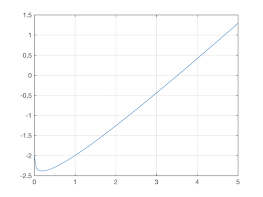
Looking at the plot we can see that $f(x)$ crosses the axis somewhere between $x=3$ and $x=4$. In other words, the solution of $f(x)=0$ is in the interval $3\le x\le4$.

2. Identify a Bracket that Contains a Root

The plot of $f(x)$ gives us the information we need to initiate an automatic root-finding procedure, for example, using the bisect function that implements the bisection algorithm. Though it is strictly not necessary, we can introduce some automation into this process with the brackPlot helper function.

Running a single statement

>> xb = brackplot('myfx',0,5)
xb =
    3.4211    3.6842

produces the following plot and stores the bracket interval in the vector, xb.

Note: Using brackPlot means that we do not generate a vector of $x$ values with x = linspace(...) and then manually plotting $f(x)$ with f =myfx(x); plot(x,f). brackPlot does that for us.

3. Refine the Guess at the Root

With a bracket to the root stored in xb, another one-line expression uses bisect to find the root.

>> r = bisect('myfx',xb)
r =
    3.5214

We store the root in r so that we can use that value later.

4. Verify that a Root Was Found

A good engineer always checks the result of a calculation. That check can be a simple "does-this-make-sense" test, or it can be an automated procedure for estimating the error in a calculation.

At the start of this root-finding example, we made a plot of $f(x)$. From that plot we saw that $f(x)$ crosses the $x$ axis between $x=3$ and $x=4$. Therefore, the value of 3.5214 returned by bisect seems like a good guess at the root.

Since the computational machinery is readily available, it always makes sense to verify the root returned by bisection. We simply evaluate

>> fr = myfx(r)
fr =
     0

In this case fr is exactly zero, which is surprising result. Normally we expect the value of $f(x)$ to be small, but not exactly zero.

We can create a visual confirmation of the root by adding the point $(r,f(r))$ to the plot created by brackPlot or to a plot created without brackPlot. Here we add the root to the plot created by `brackPlot'.

Running these statements

>> hold('on')       %  Assumes the plot is still active
>> plot(r,fr,'o')   %  Add the guess at the root
>> hold('off')

produces a plot with the root indicated by a circle.

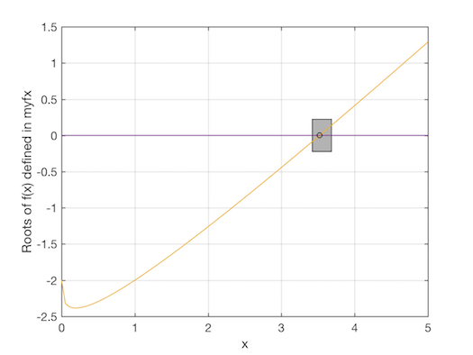
By plotting the suspected root, we confirm that $f(r)$ is small compared to the value of the function. We also see that $r$ is the location where $f(x)$ crosses the axis.

Complete MATLAB Solution

A complete MATLAB for this root-finding recipe is is listed below (download the code).

function fxroot
% fxroot  Demonstrate basic root-finding recipe with brackPlot and bisect

% -- Get possible interval with the root
xb = brackPlot('myfx',0,5);

% -- Use bisection to refine the interval
r = bisect('myfx',xb);

% -- Add the value returned by bisect for visual confirmation
hold('on')
fr = myfx(r);
plot(r,fr,'*')
hold('off')

fprintf('\nRoot found at x = %8.5f  where f(x) = %12.3e\n',r,fr)

end

Advice for using this recipe

1. First, write a simple m-file to evaluate the function $f(x)$

2. Plot $f(x)$ to visually inspect its behavior. Not all $f(x)$ are as well-behaved as the one used in this example.

3. Find a bracket to the root. You do not need to use brackPlot!

   brackPlot is a convenience function that simplifies the search for brackets. It is not fool-proof. For root-finding problems embedded in more complex analysis, you will probably want to avoid using brackPlot and instead develop a custom algorithm for guessing the roots.

4. Always test your root to make sure bisect, or whatever root-finding algorithm you are using, has found a root, not a singularity.