Using Component-analysis and System-synthesis Tools
Download the SYN tools (tarball) (zip)
either as a tar or zip archive and unpack the archive in a directory,
say "tools" in your home directory.
If you have a Windows system or a Mac, please read the file "tools/porting"
that gives advice for those platforms.
The tools are designed to be executed from a command environment.
This is a "terminal" or "command prompt" window in different systems.
If you aren't used to commands, you may want to work with system
utilities (for file creation, copying, etc.) in a graphic GUI mode.
Indeed, in Windows you may have to use the graphic utilities because
the command-line versions don't work.
The tools themselves must be run by commands.
Any application of the SYN tools takes place in a "base directory" that
contains files describing components and a system, and also the tool
scripts themselves. Perl and GNUPlot must be executable by name from
this directory. The application files that are created by hand to
describe the example are:
Executable code for each component.
Description of test subdomains for each component ("CC.ccf" for component "CC").
Description of a system to be synthesized ("system.pscf").
These files are provided in each tutorial. Understanding begins by
looking at "system.pscf", then by examining code files (though there
are better ways to study the code provided by the tools themselves).
The stateless tools are the more polished; even if you are
interested in state or concurrency, it might be
best to start with the stateless tutorial, which has the most complete
description here.
Download the component/system descriptions for the three tutorials
(tarball)
(zip)
and unpack. It is suggested that you keep the downloaded files somewhere
in separate directories
and copy them into working directories as needed; otherwise, to restore
to a pristine state you would have to download again.
Stateless-component Tutorial
The stateless tutorial is described in detail in Chapter 9 of the
monograph COMPOSING SOFTWARE COMPONENTS: A Software-testing Perspective
(Springer, 2010).
The following is a sketch of that presentation.
Copy the tutorial files to a working directory, say "TutoriaL".
If you are not particularly adept at watching multiple windows
on your screen, you might want to print out the description
you are reading now, and
have it in front of you while you run through the tutorial.
The first thing to do is to
overlay copies of
the tool scripts into the working base directory
"TutoriaL". With "TutoriaL" as the current directory
type the command:
cp ~/tools/* ./
in a UNIX/Linux/Mac system.
In Windows type:
copy ..\tools\* .
(assuming that the "tools" directory is itself in the same parent directory
as "TutoriaL"). Or copy the files
however you like to do it on your platform.
The result should be a directory "TutoriaL" containing a handful of files for the tutorial,
along with some 60-odd files from "tools", which is the current directory.
The stateless tutorial uses two components, with executable files "Math" and "Cond"
(the first is an imperative component and the second
is a conditional). But in the running version they take several
names to make each component in each position in the system unique.
"Math" is called "C1", "C3", "C5", "C6", and "C7";
"Cond" is called "T2" and "T4". You'll see these names in "system.pscf".
You should first look at these components
with the tools that would be used by a component developer to
approximate the components, "COMP" and "Xcute", which is superior
to studying the code itself.
For the tutorial a step-function approximation will be used.
Type the command:
COMP -V
which will list information about the component descriptions
and create approximate component-measurement files in "C1.ccft",
"T2.ccft", etc. Then
Xcute C1
gives you a graph of the actual and approximate behaviors for "Math" and an
error analysis. You can
guess what you type to do the same thing for "T2".
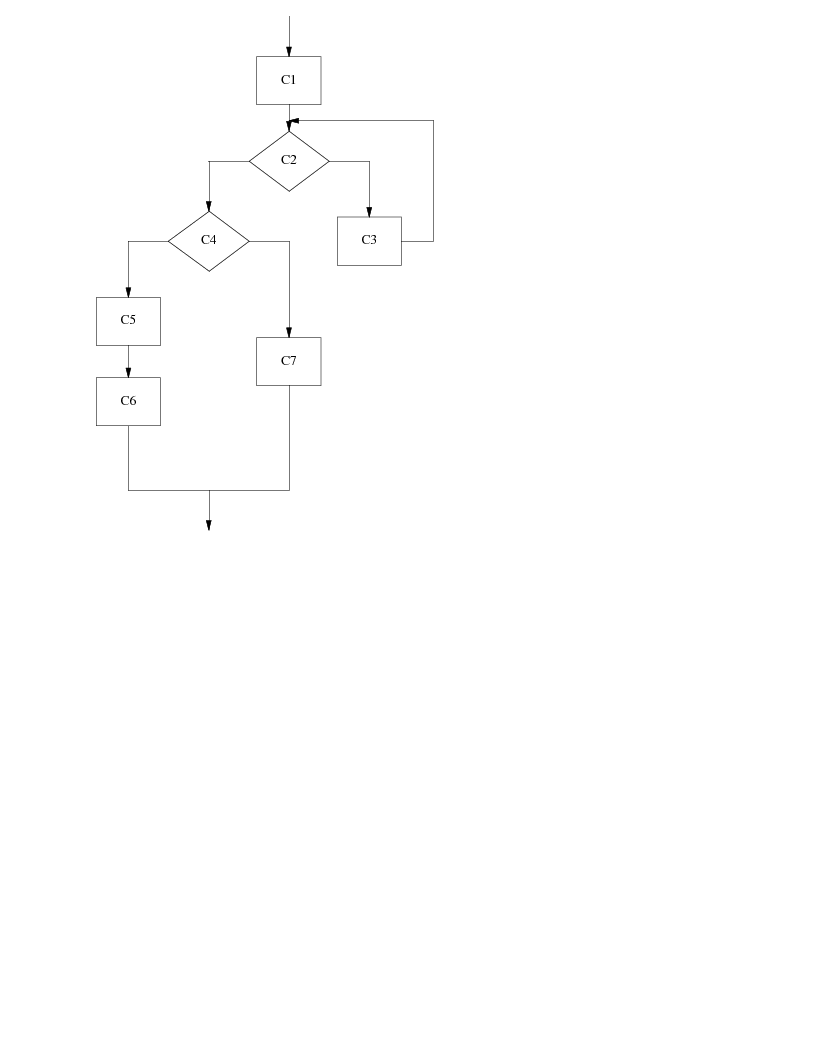
Now we are ready to synthesize a system. Look at the file "system.pscf".
It has a reverse Polish description of a system structure, which is shown
in the flowchart:

It uses seven components in this system, but really each one of them is
either "Math" or "Cond", depending on whether an imperative or conditional is
needed. If you look at the various code and .ccf files (e.g.,
"C3.ccf" and "C6.ccf"), you'll see that they are the same.
It isn't necessary to replicate same code/subdomain files in this way
unless you want to use the profile tools.
To synthesize a system, all the components have to have been approximated
first (the tools will tell you to do it if you forget).
Now to synthesize the system properties, type
SYN -V -G
and you'll see the trace of the synthesizer running, doing the reverse
Polish operators in the proper order, synthesizing equivalent components
(which it names "theory1.ccf" ... "theory5.ccf" for this example) for
the subsystems. (If you are interested in seeing what these look like,
you can use XcuteF on them later, for example
Xcute theory1
to see how the loop equivalent component behaves.
But when you look at these computed approximations there is no
comparison with actual code. If you want a comparison, it can be
had by redefining the "system" being synthesized. For example,
you could validate "theory1" by making the system consist of
just the loop, in which case the synthesis would stop after
calculating theory1.)
But right now you will see the behavior of the synthesized system
compared to the actual executed system code, with an error analysis.
There is something cool you can do here to check if the tools are working
properly. If you synthesize with
SYN -V -X -G
(adding the "-X" option),
the "actual" system that is compared to the theory calculation is built
from the approximation files ("C1.ccft", etc.), and since those are supposed
to have the approximate behavior that the theory calculates, the "theory"
and "actual" results should agree perfectly, so the error analysis
shows zero differences. (If it doesn't, you've uncovered a bug in
the tools -- not, please God, in the theory!; send an e-mail to report it.)
If you run
SYN -V -P -G
the execution will be traced. After it is complete, running
profile C6
will produce a histogram of the operational profile that appears at the
input of component C6 in the system, both measured and calculated.
You might want to study the system results in more detail, and the
Xcomp script lets you do that. (It was run for you when you used
the -G option on SYN.)
Following an execution of SYN,
Xcomp 5 9 200
(for example) displays the same error analysis and comparison graph,
but only on the
interval [5,9) and using 200 equispaced sampling points for the
actual execution. (The Xcute script has similar options.)
You could repeat the entire tutorial using the piecewise-linear
approximation by starting above with
COMP -V -L
to measure the components using a piecewise-linear
approximation.
The rest of the tutorial will be the same but
with better results.
You might want to replicate everything into a new working base directory
for such a run, especially if you want to compare the approximations
and have them both available at the same time.
To experiment with refining the subdomains, the script "splitsub 1"
can be run. It will create in the parent of the current directory
a complete new directory "TutoriaL2" which is a copy of "TutoriaL" but
with all the subdomains of all components split in two. Changing
the current directory to "Tutorial2"
and running the tools will produce results that show how
smaller subdomains improve the accuracy of measurements and
predictions.
You can now try other examples with more interesting
components. You could start by changing either the system structure
or the component behaviors in the tutorial. It is suggested that
you do so in a new directory that you first copy from "TutoriaL".
Components-with-state Tutorial
When the tools deal with components having state, the algorithms are an order of magnitude
more complicated, and they manipuate data that is quadratically more
extensive, than in the stateless case. They have been used less
for state so may be more buggy.
To try these rough-edged (or should it be "dull"?)
tools, copy the tutorial with state
into a directory (say) "TutoriaS".
Overlay the tools from "tools" into "TutoriaS".
The example system of the state tutorial is described in detail in Chapter 10
of COMPOSING SOFTWARE COMPONENTS: A Software-testing Perspective
(Springer, 2010).
The tutorial is primarily concerned with the issue of infeasible state subdomains,
which will not be covered here. However, using the tools and exploring the
example is similar to the stateless case. The components are approximated with:
COMP -V
which will give their names and subdomain descriptions.
The behavior graphs and error reports for components can be
obtained using "Xcute". To see graphs
for the component "Trig" with state, the command is:
Xcute Trig
These graphs are 2-D projections of the 3-D results as a function of
(input X state).
GNUPlot is used in its interactive mode, so the projection
surfaces for components with state can be rotated for a better view.
(Sometimes only the X-windows version of GNUPlot has this feature,
so it may be absent on your platform.)
Now you have all the components approximated.
The synthesis command is as before
SYN -V -G
which creates the files `theory1', etc. (but now with extension `.ccfc')
and an executable file named "SystemCode". (Look at
it; it just "executes" the component code files.)
The -G option displays a graphical comparison for output between calculation
and execution with an error analysis. After this has been done for the functional
system results, "Xcomp" can produce just the comparisons:
Xcomp
repeats the functional comparison, while
Xcomp -T
is for run time, and -S for state.
("Xcute" has -S and -T options as well.)
Using the -X option:
SYN -V -X -G
will compare not the actual system, but the table-lookup system
described above. For the tutorial, as in the stateless case,
there is exact agreement, but this is not always the case
for conditionals that have state in their controlled code.
The tidy system behavior graphs of the example are not the rule.
If more than one component has state, the graph becomes 4- or more
dimensional and can't be directly displayed. The tools do graph
something, but the `state' values are the vector sum of several
states, and may appear misleading.
Concurrent Components Tutorial
The example system of the concurrent tutorial is described in detail in Chapter 11
of COMPOSING SOFTWARE COMPONENTS: A Software-testing Perspective
(Springer, 2010).
The tutorial example is a `2VP' (2-Version Programming) system in which
one component starts another to process in parallel, and a non-error result is
returned only if they agree. Without going into detail, the same
"COMP", "Xcute", "SYN", and "Xcomp" commands will test, synthesize, and
display behaviors of the components and system.
As before, copy the tutorial into (say) "TutorialC" and add the tools to
this base directory, then use the commands to explore the example.
The "Master" component that starts another ("Brute") has 3-D behavior, in
which there is a second input domain of values returned by "Brute".
"Xcute -T Master" displays the run time (which can be broken into parts
throughout the interaction with options "-T1", "-T3", and "-T4".
"Xcute -O2 Master" shows what input is delivered to "Brute".
However, the slave component "Brute" and the synthesized system are
stateless, and have the usual 2-D graphs.
Last updated: May, 2010
