EE171
EE171
Electrical Engineering Department
Portland State University
Portland, OR
MENTOR TOOLS TUTORIAL SESSION #3
Douglas V. Hall
Craig Files
Electrical Engineering Department
Portland State University
P.O Box 751
Portland OR, 97207
Version C2
September 1998
INTRODUCTION
In the preceding tutorial sessions we showed you how to
access the Mentor manuals and how to draw the schematic for a
circuit. In this session we show you how to verify that the logic
and timing of the circuit are correct by simulating the circuit.
Simulation is very similar to the method you use to verify
the hardware prototype of a circuit. To verify a hardware
prototype you apply test signals to the inputs of the circuit,
then use a scope or logic analyzer to observe the input and
output signals. Likewise, when you simulate a circuit with a
simulator program, you specify a set of stimulus signals that you
want applied to the inputs of the circuit. The simulator program
then evaluates the effect these signals will have on your circuit
and displays the results as waveforms or a list. From these
waveforms you can determine if the logic and timing of your
circuit are correct.
Using a simulator is relatively easy. Most of the work
involved in simulating a circuit is the same as it is for testing
a hardware prototype: first determining a set of input stimulus
signals that will thoroughly test the circuit; and second,
predicting the correct response for this set of input signals.
At the conclusion of this session you should be able to:
- Create the Design Viewpoint for a schematic design.
- Bring up the QuickSimII simulator and the appropriate windows.
- Generate input stimulus signals for a circuit.
- Run a simulation and scale the generated waveforms as desired.
- Add probes to a circuit and rerun a simulation.
- Print a hardcopy of the simulation trace window or list
window.
- Generate a "do" file which contains a set of input stimulus
signals and use this file for a simulation.
INVOKING THE DESIGN MANAGER
- Carefully bring up the Design Manager as described at the
start of Tutorial #2. Don't forget to set the MGC_WD environment
variable to the directory which contains the spike1 circuit you
drew in Tutorial #1.
SETTING UP THE DESIGN VIEWPOINT
According to the Mentor manual a Design Viewpoint is a set
of rules used to establish the configuration of your design. The
following sequence of steps will create the proper design
viewpoint references for the QuickSimII simulator and the Logic
Modeling Corp. models.
EXAMPLE DISPLAY
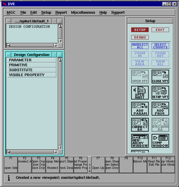
- In the Design Manager Tools window find the Design Viewpoint
Editor(DVE) icon and double click on the icon to open it.
- When the Design Viewpoint Editor window appears, find the
OPEN VPT box in the Session window on the right and click on it.
- In the Open design Viewpoint form that appears, enter
spike1 and click on OK.
EXAMPLE DISPLAY
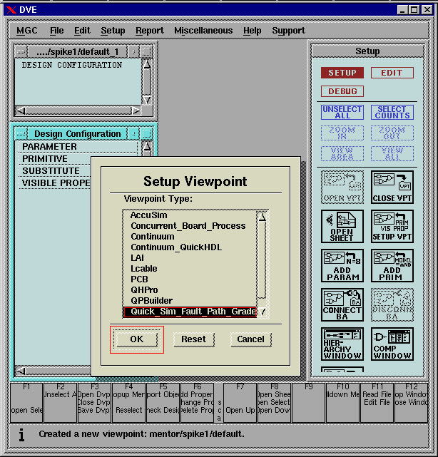
- Find the SETUP VPT in the Session window on the right and click on it.
EXAMPLE DISPLAY
- When the menu comes up, select the menu item: Quick_Sim_Fault_Path_Grade,
then press OK.
EXAMPLE DISPLAY
- When the check is completed, pop up the banner File -> Save
Design Viewpoint menu and choose With same name.
- Quit the Design Viewpoint Editor window. Then put the cursor
in the orphan command shell window, hold down the Control key,
and press the C key to get rid of this orphan.
STARTING QUICKSIM AND SETTING UP WINDOWS
- In the Design Manager Tools window, find and double click on
the QuickSimII icon to start QuickSim.
- After a short pause a form will appear. In the top box type the
path to your schematic file. (If you have set MGC_WD, all you
have to type in is spike1, otherwise you enter something like
/u/user_name/spike1).
EXAMPLE DISPLAY
In the line labeled Timing Mode click on Delay and in the line
labeled Detail of Delay Timing Mode click on Visible.
When the form expands, note that the default is typical, then
click on Max and click on OK.
- It takes the simulator a couple of minutes to generate the
netlist file, and do all the other work needed to get your
schematic ready for simulation. Eventually the QuickSim window
will appear. Grab the lower right corner of the window with the
left mouse key and drag it down and to the right to enlarge the
window.
- Read the contents of the small Model Messages window. It should
contain just a short message identifying Logic Modeling Corporation.
- Move the cursor to a blank region of the window and pop up the
QuickSim menu. You will be using this menu a lot, so read through
it to get an overview of the available commands, then choose
Open->Sheet. Eventually, an old friend should appear in a window
on the screen.
- To move the sheet view window to a more convenient location on
the screen, put the cursor in the title box containing /:sheet1,
hold down the left mouse key, use the mouse to move schematic
window to lower right corner of the QuickSim window, and
release the mouse key. (Note: If you want to move a window that
is not marked as active by a solid border, first click the left
mouse key in the title box to activate the window, then hold the
left mouse key down to move the window.)
- Activate the Model Messages window and move it down to the
lower left corner of the QuickSim window.
- The next step is to add a window which will display logic
analyzer type traces of your input stimulus signals and the
resulting output signal(s). To start, pop up the Add -> Traces
menu.
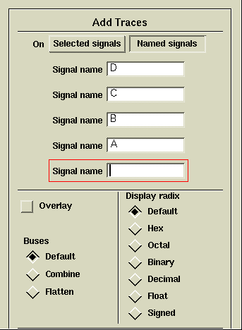
- When the Add Traces form appears, click on Named signals then
type D in the top signal name box. Type C in the next signal name
box, B in the next, A in the next, and Y in the next. Move the
cursor down until the OK button appears and click on it.
EXAMPLE DISPLAY
EXAMPLE DISPLAY
- When the Trace window appears, move it to the top of the
QuickSimII window. Note signal name labels along left side of
trace window and the time scale along the bottom. As you can see,
this window is very similar to the timing display of a logic
analyzer.
- For some circuits it is helpful to have the input and output
signals displayed in a list format as well as in waveform format.
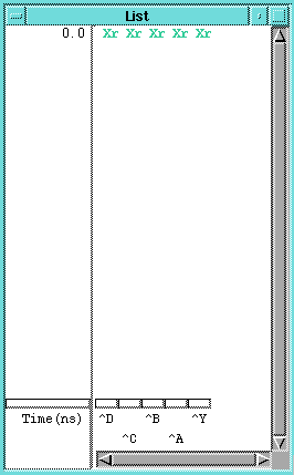
To produce a list window for this circuit pop up the Add -> List menu
and choose Specified. When the form appears, click on Named Signals,
fill in the Signal name boxes with A,B,C,D,Y, then move the cursor
down until the OK button appears and click on it.
EXAMPLE DISPLAY
- When the List window appears, move it to the left side of the
QuickSim window just below the trace window, then note the
labels in the List window.
This completes the basic setup. The next step is to create
the input stimulus signals.
CREATING INPUT STIMULUS SIGNALS
As we mentioned above, a simulator allows you to verify the
logic and the timing of a circuit. We will first show you how to
verify the logic of a circuit.
Figure 1 below shows the truth table for the spike1 circuit
you drew in session #2. To thoroughly test the logic of the
circuit you need to apply each of the possible combinations to
the inputs and check if the output is correct for each. The
sequence of input combinations is a binary count sequence, so all
you need to generate for the sequence of input stimulus signals
is a 4-bit binary counter with A as the MSB and D as the LSB.
The most common way to generate input stimulus signals in
QuickSim is with Force commands. You can force a single value
on a signal line, force a sequence of values (multiple) on a
signal line, or force a repetitive signal called a "clock" on a
signal line. The signals you need for the inputs of this circuit
are repetitive, so you will use the Add -> Force -> Clock method.
     A   B   C   D   Y
   ---------------------
     0   0   0   0   0
     0   0   0   1   0
     0   0   1   0   0
     0   0   1   1   0
     0   1   0   0   0
     0   1   0   1   1
     0   1   1   0   1
     0   1   1   1   1
     1   0   0   0   1
     1   0   0   1   1
     1   0   1   0   0
     1   0   1   1   0
     1   1   0   0   1
     1   1   0   1   1
     1   1   1   0   1
     1   1   1   1   0
Figure  1
EXAMPLE DISPLAY
- To generate a square wave signal with a 200 ns period for the
D input signal, pop up the Add -> Force -> Clock menu. When the
Force Clock form appears, type D in the Signal
Name box, type 200 in the Period box, and click on OK.
Note: The stimulus signals you create are stored in the
Waveform Data Base, but they do not appear in the trace window
until after you run the simulation.
- Repeat the procedure in #1 to generate a 400 ns square wave on
the C input, an 800 ns square wave on the B input, and a 1600 ns
square wave on the A input.
RUNNING A SIMULATION AND VIEWING THE RESULTS
- Now that you have specified the input stimulus signals, you
can run the simulation and observe the results. To run the
simulation pop up the Run -> Simulation menu and
choose Until Time. A small form should appear in the lower left
corner of the screen. One complete cycle of the input waveforms
you specified takes only 1600 ns, but to show a little extra
time, enter 2000 in the Until Time box in the form and click on
the OK button.
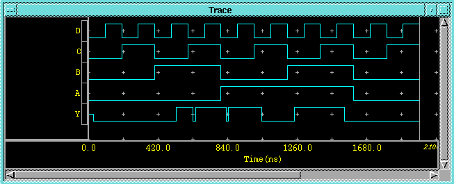
After a brief pause the input and output waveforms should
appear in the trace window and a truth table type display should
appear in the List window. Let's play around with the trace
window first.
EXAMPLE DISPLAY
- Note in the Trace window that the specified simulation stop
time is at the right side of the window. Move the cursor to the
trace window and click the left mouse key to activate that
window, then use the scroll along the bottom of the trace window
to scroll the display back to time 0.0
- Study the waveforms and observe how they correspond to the
entries in the truth table in Figure 1. Note that the value of
the Y output is indeterminate(neither high nor low) until the
applied input signals have had a chance to propagate through the
circuit. Also, note that there are a couple of glitches displayed
on the Y waveform. We will come back to these a little later.
- As with a logic analyzer display, you can change the view and
the scale of the traces. To try one of the options put the cursor
in the Trace window, pop up the View menu, study the
choices, and then choose Zoom Out -> 2.0. You should now see more
of the 2000 ns. Repeat the procedure to see the entire 2000 ns
of simulation displayed at once in the trace window.
- Use the View -> Zoom In -> 2.0 command to expand
the display until the time scale reading across the bottom has
labels for every 25 ns. Then invoke the View ->
Zoom In -> As Specified command and when the form appears in
the lower left, enter 2.5. The time scale reading across the
bottom of the screen should now have labels for every 10 ns.
- Now, suppose that you want to take a closer look at the first
glitch on the Y waveform which is at time 630 ns. You could use
the keyboard arrow keys to scroll across to that time, but an
easier way is to use the View -> Time -> Specified
command. In response to this command a small form will appear in
the lower left corner of the screen. Type 700 in the Time box of
the form. Move the cursor to one of the small arrows to the right
of "Mode relative" in the form and click the left mouse key until
absolute replaces relative in the form. Then click on the OK
button. The display should now be roughly centered on the first
output glitch. Note that the specified time of 700 is at the
right side of the screen.
Study the waveforms to determine the width of the glitch and
scroll the display so you can see the input signal transition
which causes the glitch.
- To help in examining waveforms you can add one or more
vertical cursors to the display. To do this, put the arrow cursor
in the trace window and pop up the QuickSim menu (Using the right mouse button)
and choose the Cursors -> Add command. When the form for this
command appears in the lower left, enter start as the Cursor
Name. Move the arrow cursor to the Location box, click the left
mouse key, and enter 690. Click on OK. Note that the cursor time
position is displayed at the bottom of the cursor.
EXAMPLE DISPLAY
- Once you place a cursor you can move it around anywhere you
want. Click on the vertical cursor to select it. Then pop up the
QuickSim -> Cursors menu and choose Slide. When the command
executes, a ghost of the cursor will appear. Use the mouse to
move the ghost cursor to the desired position and click the left
mouse key to place it there. Then move the arrow cursor down to
the form at the bottom of the screen and click on Cancel to
terminate the command. For practice, use a couple of cursors to
determine the time between the input transition which causes the
glitch and the end of the glitch. This is the time you have to
wait for a valid output from this circuit.
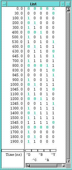
- Now let's take a look at the List window. Move the cursor to
the List window and click the left mouse key to activate the
window, then use the keyboard arrow keys to scroll to time 0.0 in
the list. Note that the list shows an entry for each time where
an input or output signal changes. Use the list entries to
determine the maximum propagation delay for the circuit.
EXAMPLE DISPLAY
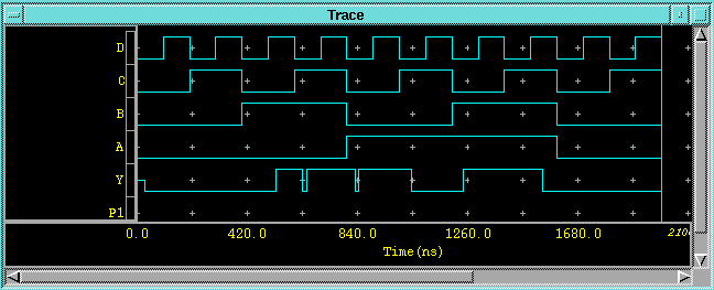
ADDING PROBES TO A CIRCUIT AND RERUNNING A SIMULATION
- Suppose you want to add a probe to output of the upper 74LS10
in the circuit so you can see a trace of the signal on that line
when you run the simulation from time 0 again. First, let's place
the probe and add a trace for it.
Move the cursor to the schematic view window and click the
left mouse key to activate the window. Put the cursor on the
output net from the upper 74LS10 and click the left mouse key to
select it. Pop up the QuickSim -> Add menu and choose Probe.
EXAMPLE DISPLAY
When the form pops up, name the probe P1, click on diamond
shaped box named Net, and then click on the OK button. When the
command executes you should see a small flag appear on the signal
line in the view window.
- To add a trace for the probe, pop up the QuickSim -> Add->
Trace menu and choose Specified. When the form pops up, click on
Named Signals, enter P1 as the signal name and click on the OK
button. An entry for P1 should appear at the left edge of the
Trace window, but there will be no trace for this probe, because
it was not present when you did the simulation.
EXAMPLE DISPLAY
NOTE: You can use the QuickSim -> Delete menu to delete a trace
and/or probe at any time.
- Now that you have the probe and trace set up, the next step is
to reset the simulator to time zero and rerun the simulation so
you can see the signal present at the point where you put the
probe.
EXAMPLE DISPLAY
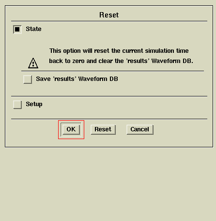
Pop up the QuickSim -> Run menu and choose Reset. When the
first form appears, click on the "state" box to choose that
option. Note: an option is chosen if the box in front of the name
contains a solid square. When the second form appears, click on
the "save results waveform DB" button to toggle this default off,
then click on the OK button. The waveforms and the cursors in the
Trace window should disappear. Also, the list in the List window
should disappear.
- To rerun the simulation, pop up the QuickSimII -> Run ->
Simulation menu and choose Until Time. When the form appears in
the lower left corner of the screen, enter 2000 as the time and
click on the OK. After a short pause new traces and a new list
should appear. Use the QuickSim -> View -> View All command to
see the traces for the entire simulation time.
EXAMPLE DISPLAY
MAKING A HARDCOPY OF THE TRACE AND LIST WINDOWS
- About now you would probably like to see some tangible results
from all your work. Let's start with a hardcopy of the trace
waveforms.
If it is not already activated, move the cursor to the trace
window and click the left mouse key to activate it. Move the
cursor to the File entry in the banner at the top of the QuickSim
window, pop up the File -> Print menu, and choose "Active
Window".
- When the form appears, you can use the default printer name
already in the printer box, or you can enter one from the list
given in Tutorial Session #2. Enter 0 as the Begin domain and 2000
as the End domain. The default scale is 1.0 which is appropriate
here, so you can leave that box blank. If you want to show the
cursors in the printout, click on the cursors box in the form.
Click on the OK button to send the trace waveforms off to the print
spooler. If the attempt is successful, you should receive a
confirmation message at the bottom of the screen.
- To make a hard copy of the list window, activate the list
window, pop up the File -> Print window and choose Active Window.
When the form appears, enter 0 as the Begin time, 2000 as
the End time, then click on OK.
RUNNING A SIMULATION WITH A FORCEFILE
The design-simulate cycle is usually repeated several times
before a final design is achieved. To save entering the force
commands individually for each simulation you can write them to a
file and then just use the file to apply the force commands when
you resimulate. Here's how you generate and use a forcefile.
- Put the cursor on the MGC entry in the banner, pop up the
Notepad menu, and choose New. NOTE: If you want to edit an
existing file, choose Open and when prompted, select the file you
want to edit from the list shown.
EXAMPLE DISPLAY
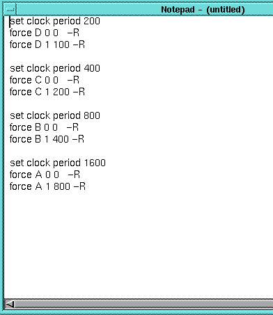
- When the notepad appears, type in the following force
commands.
set clock period 200
force D 0 0   -R
force D 1 100 -R

set clock period 400
force C 0 0   -R
force C 1 200 -R

set clock period 800
force B 0 0   -R
force B 1 400 -R

set clock period 1600
force A 0 0   -R
force A 1 800 -R
- To write this file to disk, put the cursor on the File entry
in the banner, Pop up the file menu, and choose Save As. When the
form appears enter spike1.do as the document name and click on
OK.
- To close the notepad window, put the cursor on the small box
in the upper LEFT corner of the notepad window, pop up the menu
there, and choose close.
- To reset the simulator state pop up the QuickSimII -> Run menu
and choose Reset. When the form appears, click on state, make
sure the Save waveform DB is toggled off, and click on OK.
- To eliminate the old forces from the waveform Data Base, pop
up the QuickSim -> Force menu and choose Delete. When the form
pops up, click on All Signals and click on OK.
- To apply the forces you specified in the forcefile, pop up the
QuickSimII -> Forces menu and choose From file. When the form
appears, type spike1.do, and click on OK.
- To run the simulation with these forces, pop up the
QuickSim -> Run -> Simulation menu and choose Until time.
When the form appears in the lower left corner, enter 2000, and
click on OK. After a short time the familiar simulation waveforms
should appear.
OPTIONAL PRACTICE
If you are having fun with all this and time permits, here's
a little experiment you can do for extra practice.
Using a common Karnaugh map method an engineer determined
that the ABCD input transitions 0111->0110->0111, 1110->1100-
>1110, and 1101->0101->1101 may cause static 1 hazards on the
output of the spike1 circuit you drew.
- Generate a do file which will apply these three input
sequences to the circuit.
- Reset the simulator state.
- Delete the old forces in the Waveform Data Base.
- Rerun the simulation with your new do file.
- Make a hard copy of the resulting traces
- Determine if these transitions actually do cause
hazards(glitches) on the output of the circuit.
EXITING FROM QUICKSIM
- Put the cursor in the Quicksim banner at the very top, pop
up the menu there, and choose Quit. When the form appears click
on Without Saving and click on OK.
After some time QuickSim will disappear but its command shell
window may still be present in the center of the screen. To get
rid of this, put the cursor in it, hold down the Control key
and press the C key.
- Quit from the Design Manager.