CS163 Data Structures
Week #7
Notes
Tree Structures
• Chapter 11: Tables and Priority
Queues
• Traversal of binary trees, Treesort,
Building a binary search tree
• The efficiency of searching algorithms
• Binary Tree: insertion and deletion
examples
Tree Structures
• Chapter 12: Advanced Implementation
of Tables
• Height balance, contiguous
representation of binary trees: heaps
• 2-3 Trees
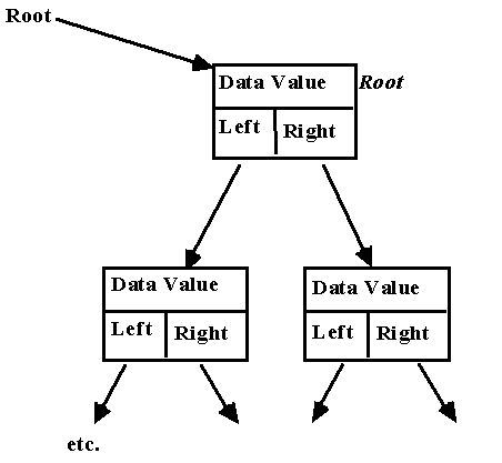
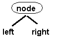
Implementing
a Binary Tree
• Just like other ADTs, we can
implement a binary tree using pointers or arrays. A pointer based
implementation example:
We
can define a tree of names as:
struct
node {
char
name[20];
node
* left_child;
node
* right_child;
};
class
binary_tree {
public:
//put
the constructor and member functions here
private:
node
* tree;
};
• If the tree is empty, tree is NULL.
• Using pointers, our binary tree
will look something like:
• Lastly, take a look at an array
based implementation to see how our binary tree could be set up. This approach
uses an array of structures. Array indices are used to indicate where the
children are located in the table.
Our
data structure would be defined as:
const
int maxnodes=100;
struct
node {
char
name[20]; //the data
int left_child; //representing an index
int
right_child; //representing an index
};
class
binary_tree {
public:
//put
the constructor and member functions here
private:
node
tree [max_nodes];
int
root;
};
When
this type of tree is empty, the Root will be zero. Otherwise, it will be the
index of where the root is located in the array. Whenever an index is zero, it
means that there is no child.
Using
this approach, as a tree changes due to inserting and deleting data, the nodes
may not be in consecutive locations in the array. Therefore, this
implementation requires that we establish some list of available nodes (we will
call this a freelist). To insert a new node into the tree, we first must obtain
an available node from the freelist. If you delete a node from the tree, you
place it into the freelist so that you can reuse the node at some later time. An array based implementation might look
something like:

Here, tree[root].left_child points
to the root of the left subtree and tree[root].right_child is the index of the
root of the right subtree.
Traversal of binary
trees
• As soon as we talk about
traversing a binary tree you should be thinking recursion! Traversal just
means visiting each node in a given tree. To begin with, lets just assume that
"visiting" a node simply means printing the data portion of the node.
• Before we create the pseudo
code, remember that a binary tree is either empty or it is in the form of a
Root with two subtrees. If the Root is empty, then the traversal algorithm
should take no action (i.e., this is an empty tree -- a "degenerate"
case). If the Root is not empty, then we need to print the information in the
root node and start traversing the left and right subtrees. When a subtree is
empty, then we know to stop traversing it.
• Given all of this, the recursive
traversal algorithm is:
Traverse
(Tree)
If
the Tree is not empty then
Print
the data at the Root
Traverse(Left
subtree)
Traverse(Right
subtree)
• But, this algorithm is not
really complete. When traversing any binary tree, the algorithm should have 3
choices of when to process the root: before it traverses both subtrees (like
this algorithm), after it traverses the left subtree, or after it traverses
both subtrees. Each of these traversal methods has a name: preorder, inorder, postorder.
• You've already seen what the
preorder traversal algorithm looks like...it would traverse the following tree
as: 60,20,10,5,15,40,30,70,65,85
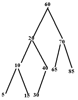
• The inorder traversal algorithm
would be:
Traverse
(Tree)
If
the Tree is not empty then
Traverse(Left
subtree)
Print
the data at the Root
Traverse(Right
subtree)
• It would traverse the same tree
as: 5,10,15,20,30,40,60,65,70,85; Notice that this type of traversal produces
the numbers in order. Search trees can be set up so that all of the nodes in
the left subtree are less than the nodes in the right subtree.
A
treesort is simply a method of taking the items to be sorted, building a binary
search tree, and then traversing it inorder to put them in order. This solves
the problems we have encountered of inserting or deleting items in a contiguous
list -- or having to sequentially traverse a linked list (both of which can be
very inefficient).
• The postorder traversal algorithm
would be:
Traverse
(Tree)
If
the Tree is not empty then
Traverse(Left
subtree)
Traverse(Right
subtree)
Print
the data at the Root
• It would traverse the same tree
as: 5, 15, 10,30,40,20,65,85,70,60
• Think about the code to traverse
a tree inorder using a pointer based
implementation:
void
inorder_print(binary_tree tree) {
if
(tree) {
inorder_print(tree->left_child);
cout
<<tree->name);
inorder_print(tree->right_child);
}
• As an exercise, try to write a
nonrecursive version of this!
ADT
Table Operations -- using a binary search tree
• We can implement our ADT Table
operations using a nonlinear approach of a binary search tree. This provides
the best features of a linear implementation that we previously talked about plus
you can insert and delete items without having to shift data. You can locate
items by using a binary search-like algorithm. With a binary search tree we are
able to take advantage of dynamic memory allocation.
• Linear implementations of ADT table operations are still useful.
Remember when we talked about efficiency, it isn't good to overanalyze our
problems. If the size of the problem is small, it is unlikely that there will
be enough efficiency gain to implement more difficult approaches. In fact, if
the size of the table is small using a linear implementation makes sense
because the code is simple to write and read!
• For test operations, we must
define a binary search tree where for each node -- the search key is greater
than all search keys in the left subtree and less than all search keys in the
right subtree. Since this is implicitly a sorted tree when we traverse it
inorder, we can write efficient algorithms for retrieval, insertion, deletion,
and traversal. Remember, traversal of linear ADT tables was not a
straightforward process!
Let's
quickly look at a search algorithm for a binary search tree implemented using
pointers (i.e., implementing our Retrieve ADT Table Operation):
The
following is pseudo code:
void
retrieve (binary_tree *tree, int key, int & returneddata, int success) {
if (!tree) //we
have an empty tree
success =0;
else if (tree->data == key) { //we have found the node we are looking
for
success = TRUE;
returneddata =
Tree->data;
}
else if (key < tree->data) //look down the left branch
retrieve(tree->left_child, key,
returneddata, success)
else //look
down the right branch
retrieve(tree->right_child, key,
returneddata, success)
}
• To traverse such a tree, we
simply need to use inorder traversal.
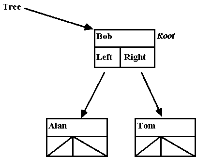
• Now, write the pseudo code to
insert:
Insert(Tree,NewItem)
• In this pseudo code it is
important that Tree be able to be changed. When it is set to point to the new
structure, the effect is to set the previous' Left or Right pointer to point to
this new structure. Let's start with:
and, insert Frank:
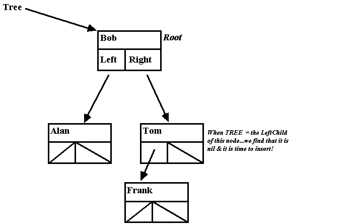
• You can create a binary search
tree by using Insert and starting with an empty tree. Then, it will insert
names in the proper order.
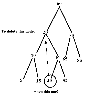
• Lastly, think about
deleting an item. It ends up not being as simple as the other two operations we
have looked at. Why? Because we need to consider three special cases: When we
are deleting a leaf, when we are deleting a node which has 1 child, and when we
are deleting a node which as two children.
The
first case is the easiest. To remove a leaf we simply change the Left or Right
pointer in its parent to NULL. In the second case, we end up letting the parent
of the node to be deleted adopt the
child! It ends up not making a difference if the child was a left or a right
child to the node being deleted.
The
third case is the most difficult. Both children cannot be "adopted"
by the parent of the node to be deleted...this would be invalid for a binary
search tree. The parent has room for only one of the children to replace the
node being deleted. So, we must take on a different strategy. One way to do
this is to not delete the node; instead replace the data in this node with
another node's data...it can come from immediately after or before the search
key being deleted.
How can a node with a key matching this
description be found? Simple. Remember that traversing a tree INORDER causes us
to traverse our keys in the proper sorted order. So, by traversing the binary
search tree in order, starting at the to-be-deleted node (i.e., the
to-be-replaced node)...we can find the search key to replace the deleted node
by traversing the next node INORDER. It is the next node searched and is called
the inorder successor. Since we know
that the node to be deleted has two children, it is now clear that the inorder
successor is the leftmost node of the "deleted nodes" right subtree.
Once it is found, you copy the value of the item into the node you wanted to
delete and remove the node found to replace this one -- since it will never
have two children.
Height
& Balance -- binary trees
• We already know that the maximum
height of a binary tree with N nodes is a height of N. And, an N-node tree with
a height of N resembles a linked list.
• It is interesting to consider
how many nodes a tree might have given a certain height. If the height is 3,
then there can be anywhere between 3 and 7 nodes in the tree. Trees with more
than 7 nodes will require that the height be greater than 3. A full binary tree
of height h -- should have 2h-1 nodes in that
tree
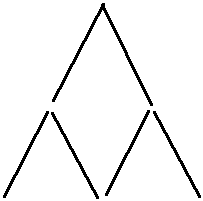
• Look at a diagram ... counting
the nodes in a full binary tree
A full binary tree of height at
Level 1: # of nodes = 21-1 =
1
A full binary tree of height at
Level 2: # of nodes = 22-1 = 3
A full binary tree of height at
Level 3: # of nodes = 23-1 = 7
• We are now ready to examine what
we need to do to find the minimum height of a binary tree with N nodes. It is log2(N+1)
-- rounded up (ceiling). To find the minimum height of a binary tree,
we know that a full binary tree of height h
has 2h-1 nodes. Therefore,
if a binary search tree is balanced -- and therefore complete -- the time it
takes to search it for a value is about the same as is required by a binary
search of an array. The height of a binary search tree can range anywhere
between a maximum height of N to a
minimum height of log2(N+1).
Heaps
• A heap is a data structure
similar to a binary search tree. However, heaps are not sorted as binary search
trees are. And, heaps are always complete binary trees. Therefore, we always
know what the maximum size of a heap is.
• Unlike a binary search tree, the
value of each node in a heap is greater than or equal to the value in each of
its children. In addition, there is no relationship between the values of the
children; you don't know which child contains the larger value. Heaps are used
to implement priority queues.
• A priority queue is an Abstract
Data Type! Which, can be implemented using heaps. Think of a To-Do lists; each
item has a priority value which reflects the urgency with which each item
needed to be addressed. By preparing a priority queue, we can determine which
item is the next highest priority. A priority queue maintains items sorted in
descending order of their priority value -- so that the item with the highest
priority value is always at the beginning of the list.
• Priority Queue ADT operations
can be implemented using heaps..which is a weaker binary tree but sufficient for
the efficient performance of priority queue operations. Let's look at heap:
• To remove an item from a heap,
we remove the largest item (or the item with the highest priority). Because the
value of every node is greater than or equal to that of either of its children,
the largest value must be the root of the tree. A remove operation is simply to
remove the item at the root and return it to the calling routine.
Once
you have removed the largest value, you are left with two disjoint heaps: 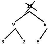
Therefore,
you need to transform the nodes that remain after the root is removed back into
the heap. To begin this transformation, take the item in the last node of the
tree and place it in the root. Notice we can't just pick the greater of 9 or 6 in the root, because we must be careful to make sure we always
have a complete tree! Therefore, we place the last node in the root and then
take that value and trickle it down the tree until it reaches a node in which
it will not be out of place. The value will come to rest in the first node
where it would be greater than (or equal to) the value of each of its children.
To accomplish this, first compare the new value in the root to each of its
children; if the root's value is smaller than the values of both of its
children, swap the item in the root with that of the larger child....which
means the child whose value is greater than the value of the other child. Let's
see how this works:
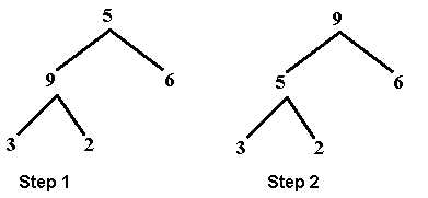
Even
though only one swap was necessary here to trickle 5 down, usually more swaps are necessary....and can follow a
recursive algorithm. Notice the result is still a complete binary tree!
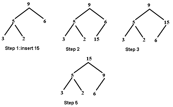
• To insert an item, we use just
the opposite strategy. We insert at the bottom of the tree and trickle the
number upward to be in the proper place. With insert, the number of swaps
cannot exceed the height of the tree -- so that is the worst case! Which, since
we are dealing with a binary tree, this is always approximately log2(N)
which is very efficient.
• The real advantage of a heap is
that it is always balanced. It makes a heap more efficient for implementing a
priority queue than a binary search tree because the operations that keep a
binary search tree balanced are far more complex than the heap operations.
However, heaps are not useful if you want to try to traverse a heap in sorted
order -- or retrieve a particular item.
Heapsort
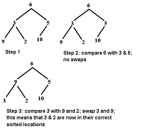
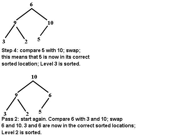
• A heapsort uses a heap to sort a
list of items that are not in any particular order. The first step of the
algorithm transforms the array into a heap. We do this by inserting the numbers
into the heap and having them trickle up...one number at a time.
A
better approach is to put all of the numbers in a binary tree -- in the order
you received them. Then, perform the algorithm we used to adjust the heap after
deleting an item. This will cause the smaller numbers to trickle down to the
bottom. See how this works:
Advanced
Implementations of the ADT Table
• Using balanced search trees, we
can achieve a high degree of efficiency for implementing our ADT Table
operations. This efficiency depends on the balance of the tree. We will find
that balanced trees can be searched with efficiency comparable to the binary
search.
• With a binary search tree, the
actual performance of Retrieve, Insert, and Delete actually depends on the
tree's height. Why? Because we must follow a path from the root of the tree
down to the node that contains the desired item. At each node along the path,
we must compare the key to the value in the node to determine which branch to
follow. Because the maximum number of nodes that can be on any path is equal to
the height of the tree, we know that the maximum number of comparisons that the
table operations can require is also equal to the height.
• Now let's take a look at some
factors that determine the height of a binary search tree. The height is
affected by the order of the data picked to be inserted and deleted. If we had
the numbers: 10, 20, 30, 40, 50, 60, 70...and inserted them in ascending order,
we would get the tree shown on the left (which has maximum possible height).
If, we inserted the items as: 40, 20, 60, 10, 30, 50, 70...we would get a
search tree of minimum height (shown on the right):
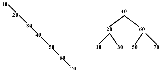
• Trees that have a linear shape
behave no better than a linked list. Therefore, it is best to use variations of
the basic binary search tree together with algorithms that can prevent the
shape of the tree form degenerating. Two variations are the 2-3 tree and
the AVL tree.
• One reason we will focus on the
2-3 tree is that a generalization of the 2-3 is called a B-tree which is a data structure that we can use to implement a
table that resides in external memory.
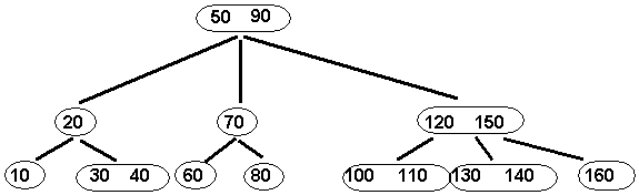
2-3
Trees
• 2-3 trees permit the number of
children of an internal node to vary between two and three. This feature allows
us to "absorb" insertions and deletions without destroying the tree's
shape. We can therefore search a 2-3 tree almost as efficiently as you can
search a minimum-height binary search tree...and it is far easier to maintain a
2-3 tree than it is to guarantee a binary search tree having minimum height.
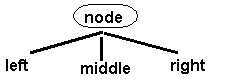
• Every node in a 2-3 tree is
either a leaf, or has either 2 or 3 children. So, there can be a left and right
subtree for each node...or a left, middle, and right subtree.
• To use a 2-3 tree for
implementing our ADT table operations we need to create the tree such that the
data items are ordered. The ordering of items in a 2-3 search tree is similar
to that of a binary search tree. In fact, you will see that to retrieve -- our
pseudo code is very similar to that of a binary search tree.
• The big difference is that nodes
can contain more than one set of data. If a node is a leaf, it may contain
either one or two data items! If a node has two children, it must only contain
1 data item. But, if a node has three children, it must contain 2 data items.
• When we have the case:
• Then, the "node"
contains only one data item. In this case, the value of the key at the
"node" must be greater than the value of each key in the left subtree
and smaller than the value of each key in the right subtree. The left and right
subtrees must each be a 2-3 tree.
• When we have the case:
• Then, the "node"
contains two data items. In this case, the value of the smaller key at the
"node" must be greater than the value of each key in the left subtree
and smaller than the value of each key in the middle subtree. The value of the
larger key at the "node" must be greater than the value of each key
in the middle subtree and smaller than the value of each key in the right
subtree. The left, middle, and right subtrees must each be a 2-3 tree.
• Now, think about the pseudocode
to retrieve an item from such a tree:
Retrieve
(Tree, Key, Returneddata,Success)
• Now think about how we could
traverse a 2-3 search tree in sorted order:
Inorder
(Tree)
• With insertions, since the nodes
of a 2-3 tree can have either 2 or 3 children and can contain 1 or two data
values -- we can make insertions while maintaining a tree that has a balanced
shape. That is the goal!
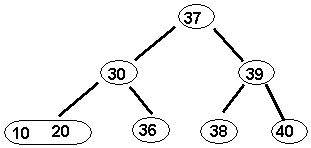
Say
we start with a tree that looks like:
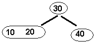
and,
we want to insert 39. The first step
is to locate the node where a search for 39 (if it was in the tree) would
terminate. This is the same as the approach we just discussed to retrieve an
item from a tree; we would terminate at node 40. Since this node contains only 1 item, you can simply insert the
new item into this node. Here is the result:
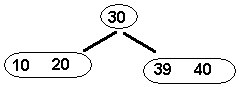
Now,
insert 38. Again, we would search
the tree to see where the search will terminate if we had tried to find 38 in
the tree...this would be at node <39
40>. Immediately we know that nodes contain 1 or 2 data items...but NOT
THREE! So, we can't simply insert this new item into the node.
Instead,
we find the smallest (38), middle (39) and largest (40) data items at this
node. You can move the middle value (39) up to the node's parent and separate
the remaining values (38,40) into two nodes attached to the parent. Notice that
since we moved the middle value to the parent -- we have correctly separated
the values of its children. See the results:
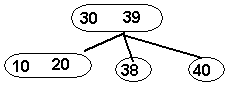
Now,
insert 37. This is easy because it
belongs in a leaf that currently contains only 1 data value (38). The result
is:
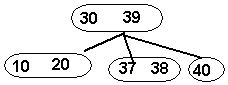
Now,
insert 36. We find that this number
belongs in node <37 38>. But,
once again we realize that we can't have 3 values at a node...so we locate the
smallest (36), middle (37), and largest (38) values. We then move the middle
value (37) up to the parent and attach to the parent two nodes (the smallest
and the largest).
However,
notice that we are not finished. We have now tried to move 37 to the parent --
trying to give it 3 data items (think recursion!!) -- and trying to give it 4
children! As we did before, we divide the node into the smallest (30), middle
(37), and largest (39) values...and move the middle value up to the node's
parent.
Because
we are splitting a node, we must take care of its children. We should attach
the left pair of children <10,20>
and <36> to the smallest value (30), and
the right pair of children <38> and <40> to the largest
value <39>. The result is:
• So, here is the insertion
algorithm. To insert a value into a 2-3 tree we first must locate the leaf
which the search for such a value would terminate. If the leaf only contains 1
data value, we insert the new value into the leaf and we are done.
However,
if the leaf contains two data values, we must split it into two nodes (this is
called splitting a leaf). The left node gets the smallest value and the right
node gets the largest value. The middle value is moved up to the leaf's parent.
The new left and right nodes are now made children of the parent.
If
the parent only had 1 data value to begin with, we are done. But, if the parent
had 2 data values, then the process of splitting a leaf would incorrectly make
the parent have 3 data values and 4 children! So, we must split the parent
(this is called splitting an internal node). You split the parent just like we
split the leaf...except that you must also take care of the parent's four
children. You split the parent into two nodes. You give the smallest data item
to the left node and the largest data item to the right node. You attach the
parent's two leftmost children to this new left node and the two rightmost
children to the new right node. You move the parent's middle data value to it's
parent..and attaching the left and right newly created nodes to it as its two
new children.
This
process continues...splitting nodes...moving values up recursively until a node
is reached that only has 1 data value before the insertion.
The
height of a 2-3 tree only grows from the top. An increase in the height will
occur if every node on the path from the root of the tree to the leaf where we
tried to insert an item contains two values. In this case, the recursive
process of splitting a node and moving a value up to the node's parent will
eventually reach the root. This means we will need to split the root. You split
the root into two new nodes and create a new node that contains the middle
value. This new node is the new root of the tree.