CS163 Data Structures
Week #4
Notes
Other Lists and
Their Implementation
• Linked Lists: dynamic memory
allocation and pointers
• Variations of the Linked List
Algorithm Efficiency and Searching
• Chapter 9 - Algorithm Efficiency and
Sorting
• Measuring efficiency of algorithms:
order of magnitude analysis, Big O notation
• Chapter 2 Searching for Things
(page 81)
Remember: Sequential
search, binary search
• Evaluating the efficiency of the
algorithms
Variations
of the Linked List
• With a linked list,
if we want to access the first node of a linked list after accessing the last
node, we must go back and look at the head pointer. But, instead, when this is
an operation common to our application, we could simply change the next field of the list's last node to
point to the head of the list instead of containing NULL. The result is a circular
linked list!
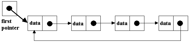
• With a circular
linked list, you can start anywhere in the list and be able to traverse the
entire list. You would still need an external pointer, pointing to where you
want to normally start traversing.
• With a circular
linked list, if you ever encounter a pointer that is NULL, that can ONLY mean
that the list is empty! Notice that no node in a circular list contains NULL in
its next field. Otherwise it wouldn't be circular!! Therefore, traversal
algorithms must change. We can't traverse our list until we encounter a NULL
pointer! Instead, we simply compare the current pointer (what we are using to
step thru the list with) -- to the external pointer which points to the first
item in the list. If they are the same, we know that we have traverse the
entire list!
• Many times, the
first pointer will actually be set to the "last node"! This way we
can quickly access both the first and last nodes without ever doing any
traversal: list->link points to
the first node and list points to the
last node. list->link->data is
the data item of the first node:
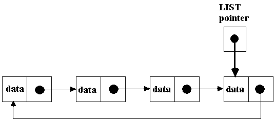
• Given this approach,
the following is the pseudo code to write the data fields of every node in a
circular list, assuming that list
points to the "last" node.
if (list != NULL) //make sure that the list is not empty
{
current = list; //use a "current pointer" to step
thru the list
do {
current =
current->link;
cout
<<current->data <<endl;
} while (current != list)
}
• On your own, try to
write the routines to insert and delete from a circular linked list!
Avoiding
Special Casing our Linked Lists.....
• Another interesting
concept is that we can modify our linked list algorithm to avoid special casing
the FIRST NODE for insertion and deletion!
Although we can write algorithms
to correctly handle these cases, many times our code is clearer if we can deal
with all nodes in the same manner. One method to do this is to have a dummy head node. Let's look at a
picture of this:
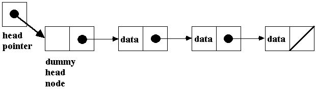
• Using this method,
the item at the first position of the list is actually the second node! When
you use a dummy head node, there is no special case in the insert and delete
functions because they will initialize our previous pointer -- to point to the
dummy head node rather than to NULL.
• Sometimes, people use the dummy
node to actually store vital information about your list. Like its length, the
smallest data item, the largest data item, etc. We might declare our list to
have a "head" structure to contain this information, instead of using
a dummy or empty node:
struct node {
int data;
node * link;
};
struct head {
int length;
int smallest;
int largest;
node *first_item;
};
class list {
public:
//member functions
private:
head * list_ptr; //points to the head structure
};
In this case, what would your constructor
look like?
Think about list_ptr...does it really need
to be a pointer?
Algorithm Efficiency
• If
we say: Algorithm A requires a certain
amount of time proportional to f(N)...this means that regardless of the
implementation or computer, there is some amount of time that A requires to
solve the problem of size N. Algorithm A is said to be order f(N) which is denoted as O(f(N));
f(N) is called the algorithm's growth-rate function. We call this
the BIG O Notation!
•
Examples of the Big O Notation:
If a problem requires a constant time that
is independent of the problem's size N, then the time requirement is defined
as: O(1).
If a problem of size N requires time that
is directly proportional to N, then the problem is O(N). If the time
requirement is directly proportion to Nsquared, then the problem is
O(Nsquared), etc.
• Some
things to keep in mind when using this notation.
You can ignore low-order terms in an
algorithm's growth rate. For example, if an algorithm is O(N3+ 4*N2+3*N)
then it is also O(N3). Why? Because N3is significantly
lager than either 4*N2 or 3*N...especially when N is large. For
large N values...the growth rate of N3+ 4*N2+3*N is the
same as N3
•
Also, you can ignore a constant being multiplied to a high-order term. For
example: if an algorithm is O(5*N3), then it is the same as O(N3).
•
Lastly, one algorithm might require different times to solve different problems
that are of the same size. For example, searching for an item that appears in
the first location of a list will be finished sooner than searching for an item
that appears in the last location of the list (or doesn't appear at all!).
Therefore, when analyzing algorithms, we should consider the maximum amount of
time that an algorithm can require to solve a problem of size N -- this is
called the worst case. Worst case
analysis concludes that your algorithm is O(f(N)) in the worst case.
• You
might also consider looking at your algorithm time requirements using average case analysis. This attempts to
determine the average amount of time that an algorithm requires to solve
problems of size N. In general, this is far more difficult to figure out than
worst case analysis. This is because you have to figure out the probability of
encountering various problems of a certain size and the distribution of the
type of operations performed. Worst case analysis is far more practical to
calculate and therefore it is more common.
• The
next step is to learn how to figure out an algorithm's growth rate. We know how
to denote it...and we know what it means (i.e., usually the worst case) and we
know how to simplify it (by not including low order terms or constants)...but
how do we create it?
• Here
is an example of how to analyze the efficiency of an algorithm to traverse a
linked list...using the following code:
void printlist(node *head)
{
node * cur;
cur = head;
while (cur != NULL) {
cout
<<cur->data;
cur = cur->link;
}
}
• If
there are N nodes in the list; the number of operations that the function
requires is proportional to N. For
example, there are N+1 assignments and N print operations, which together are
2*N+1 operations. According to the rules we just learned about, we can ignore
both the coefficient 2 and the constant 1; they are meaningless for large
values of N. Therefore, this algorithm's efficiency can be denoted as O(N); the
time that printlist requires to print N nodes is proportional to N. This makes
sense: it takes longer to print or traverse a list of 100 items than it does a
list of 10 items.
•
Another example, using a nested loop:
for (i=1; i <= n; i++)
for (j=1; j <=n; j++)
x = i*j;
This is O(n squared)
• The
concepts learned here can also be used to help choose the type of ADT to use
and how efficient it will be. For example, when considering whether to use
arrays or linked lists, you can use this type of analysis...since there may be
significant difference in the efficiency between the two!
•
Take, for example, the ADTs for the ordered list operation RETRIEVE; remember,
it retrieves a value of the item in the Nth position in the ordered list.
In the array based implementation, the Nth
item can be accessed directly (it is stored in position N). This access is
therefore INDEPENDENT OF N! Therefore, RETRIEVE takes the same amount of time
to access either the 100th item or the first item in the list. Thus, an array
based implementation of RETRIEVE is O(1).
In the pointer based implementation (using
a linked list), we must traverse the list from its beginning until the Nth node
is reached. Like the previous printlist algorithm, RETRIEVE is O(N).
•
Whenever you are analyzing these algorithms, it is important to keep in mind
that we are only interested in significant differences in efficiency. Can
anyone tell me if the difference in efficiency for the two implementations of
RETRIEVE are significant????
Notice that as the size of the list grows,
the pointer base implementation might require more time to retrieve the desired
node (it definitely would in the worst case situation...because the node is
farther away from the beginning of the list). In contrast, regardless of how
large the list is, the array based implementation will always require the same
constant amount of time.
Therefore, the difference in efficiency is
worth considering if your problem is large enough. However, if your list never
has more than a few items in it, the difference is not significant!
• There
is one side note that we should consider. When evaluating an algorithm's
efficiency, we always need to keep in mind the trade-offs between execution
time and memory requirements. The Big O notation is denoting execution time and
does not fill us in concerning memory requirements and/or algorithm
limitations. So, once you find out about performance time, you need to include
thoughts about how much memory one approach requires over another and the
strengths/weaknesses of the algorithms themselves (are there certain cases that
are not handled effectively?).
•
Overall, it is important to examine your algorithms for both style and
efficiency. If your problem size is small, don't over analyze; pick the
algorithm easiest to code and understand. Sometimes less efficient algorithms
are more appropriate.
Searching
• The ADT's we have
learned about so far are appropriate for problems that must manage data by the position of the data (the ADT operations for an Ordered List,
Stack, and Queue are all position oriented). These operations insert data
(at the ith position, the top of stack, or the rear of the queue); they delete
data (at the ith position, the top of stack, or the front of the queue); they
retrieve data and find out if the list is full or empty.
• Tables, on the other
hand, manage data by its value! As
with the other ADT's we have talked about, table operations can be implemented
using arrays or linked lists.
• Valued Oriented ADTs allow you to:
-- insert data containing a certain VALUE
into a data structure
-- delete a data item containing a certain
VALUE from a data structure
-- retrieve data and find out if the
structure is empty or full.
• Applications that
use value oriented ADTs are:
...finding the phone number of John Smith
...deleting all information about an
employee with an ID # 4432
• For those of you who
took CS162 from me...you should immediately think of our project and how we
searched for items in a data base of information ... printed it and/or deleted
it. Thus, we used the concept of value oriented ADTs without ever knowing it.
Now let's expand that to actually IMPLEMENTING such capabilities using ADT
Table operations!
• When you think of an
ADT table, think of a table of major cities in the world including the
city/country/population, a table of To-Do-List items, or a table of addresses
including names/addresses/phone number/birthday. Each entry in the table
contains several pieces of information. It is designed to allow you to look up
information. You can find out what the population is of London, find out what
all of the high-priority To-Do-List items are, or find out the telephone number
of everyone whose birthday occurs this month.
• And, with Tables, we can look up
information easily in any category. For example:
City Country Population
Athens Greece 2,500,000
Cairo Egypt 9,500,000
London England 9,400,000
NewYork USA 7,300,000
Rome Italy 2,800,000
Toronto Canada 3,200,000
Venice Italy 300,000
We
could pick any city and find out the country and population. Or, we could pick
any country and find all of the cities and their corresponding populations. Or,
we could find all cities with populations less than 1 million.
• Obviously, to do
this we would use structures for our data...since our data is more complex than
a simple integer or real number.
• The basic operations
that define an ADT Table are:
• Create an empty table (e.g., Create(Table))
• Insert an item into the table (e.g., Insert(Table,Newdata))
• Delete an item from the table (e.g., Delete(Table, Key))
• Retrieve an item from the table (e.g., Retrieve(Table, Key, Returneddata))
• But, just like
before, you should realize that these operatons are only one possible set of
table operations. Your application might require either a subset of these
operatons or other operations not listed here. Or, it might be better to modify
the definitions...to allow for duplicate items in a table.
• Does anyone see a
problem with this approach so far? What if we wanted to print out all of the
items that are in the table? Let's add a traverse.:
• Traverse the Table (e.g., Traverse(Table, VisitOrder))
Traverse simply visits every item in the
table. It should be given some clue as to how to traverse the list; for
example, traversal will be performed by specifying the field you want to step
through in sorted order (alphabetically by city, alphabetically by country, or
by population size).
• Given these ADT
operations...what would we do if we wanted to print, in alphabetical order, the
name of each city and its population?
Linear
Implementation of the ADT Table
• We will look at both
array based and pointer based implementations of the ADT Table. When we say
linear, we mean that our items appear one after another...like a list. Linear
lists are very appropriate for tables. The following shows the format for two
different linear lists:
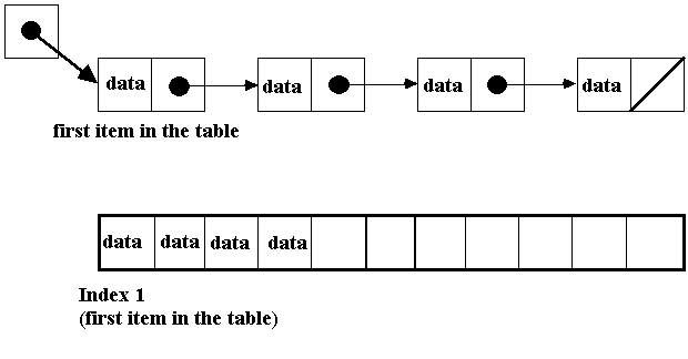 (Notice that the data is each a
structure of information)
(Notice that the data is each a
structure of information)
• With these tables,
we can either organize them in sorted order or not. If your application
frequently needs a key accessed in sorted order, then they should be stored
that way. But, if you access the information in a variety of ways, sorting may
not help! With an unsorted table, we can save information at the end of the
list or at the beginning of the list; therefore, insert is simple to implement:
for both array and pointer-based implementations.
For an unsorted table, it will take the
same amount of time to insert an item regardless of how many items you have in
your table. And, the only advantage of using a pointer-based implementation is
if you are unable to give a good estimate of the maximum possible size of the
table. Keep in mind that the space requirements for an array based
implementation are slightly less than that of a pointer based
impelmentation....because no explicit pointer is stored.
For sorted tables (which is most common),
we organize the table in regard to one of the fields in the data's structure.
Generally this is used when insertion and deletion is rare and the typical operation
is traversal (i.e., your data base has already been created and you want to
print a list of all of the high priority items). Therefore, the most frequently
used operation would be the Traverse operation, sorting on a particular key.
For a sorted list, you need to decide:
• Whether dynamic memory is needed
or whether you can determine
the maximum size of your table
• How quickly do items need to be
located given a search key
• How quickly do you need to insert
and delete
So, have you noticed that we have a
problem for sorted tables? Having a dynamic table requires pointers. Having a
good means for retrieving items requires arrays. Doing alot of insertion and
deletion is a toss up...probably an array is best because of the searching. So,
what happens if you need to DO ALL of these operations?
Searching Review
• Searching is
considered to be "invisible" to the user. It doesn't have input and
output the user works with. Instead,
the program gets to the stage where searching is required and it is performed.
• In many
applications, a significant amount of computation time is spent sorting data or
searching for data. Therefore, it is really important that you pick an
efficient algorithm that matches the tasks you are trying to perform. Why?
Because some algorithms to sort and search are much slower than others,
especially when we are dealing with large collections of data.
• When searching, the
fields that we search to be able to find a match are called search keys (or, a key...or a target).
Searching algorithms may be designed to search for any occurrence of a
key, the first occurrence of a key, all occurrences of a key, or the last
occurrence of a key. To begin with, our searching algorithms will assume only
one occurance of a key.
• Searching is either
done internally or externally. Searching internally means
that we will search an list of items for a match; this might be searching an
array of data items, an array of structures, or a linked list. Searching
externally means that a file of data items needs to be searched to find a
match.
• Searching algorithms
will typically be modularized into their own function(s)...which will have two
input arguments:
(1) The key to search for (target)
(2) The list to search
and, two output arguments:
(1) A boolean indicating success or
failure (did we find a match?)
(2) The location in the list where the
target was found; generally
if the search was not successful the
location returned is
some undefined value and should not
be used.
Sequential Search
•
The most obvious and primitive way to search for a given key is to start at the
beginning of the list of data items and look at each item in sequence.
•
This is called a sequential search; it is also called a linear search.
•
Suppose we have an array of integers; this algorithm is going to search through
6 keys to find a match:
Search Pattern: 17
Array: 4, 40, 7, 10, 6, 17, 21, 28,
35, 13
Where, Key[1] => 4; Key[2] =>
40; ...Key[6] => 17
•
With this algorithm, we found the first occurrence of 17.
•
The sequential search quits as soon as it finds a copy of the search key in the
array. If we are very lucky, the very first key examined may be the one we are
looking for. This is the best possible case.
•
In the worst case, the algorithm may search the entire search area - from the
first to the last key before finding the search value in the last element -- or
finding that it isn't present at all. In either of these cases, there are as
many comparisons of keys as there are elements in the search area of the list.
• In general, your performance will be somewhere between the best and the worst cases. The average search will go halfway through the list.
Binary Search
• For a faster way to
perform a search, you might instead select the binary search algorithm. This is
similar to the way in which we use either a dictionary or a phone book.
• For example, our
pseudo code to search for something in a dictionary might look like:
• Open the dictionary to a point near the
middle
• Determine which half of the dictionary
contains the word
• If the word is in the first half of the
dictionary then
Search the first half of
the dictionary for the word
Otherwise,
Search the second half
of the dictionary for the word
• As you should know
from CS162, this method is one which divides and conquers. We divide the list
of items in two halves and then "conquer" the appropriate half! You
continue doing this until you either find a match or determine that the word
does not exist!
• Thinking about
binary search, we should notice a few facts:
#1) The binary search is NOT good for
searching linked lists. Because it requires jumping back and forth from one end
of the list to the middle; this is easy with an array but requires tedious
traversal with a linear linked list.
#2) The binary search REQUIRES that your
data be arranged in sorted order! Otherwise, it is not applicable.