Quick Links:
Quick Intro Notes:
Lectures:
Last updated at 10:12 PM on 04 Mar 2009
![]() Subscribe to the
RSS feed for lecture podcasts.
Subscribe to the
RSS feed for lecture podcasts.
This page provides learning objectives and other supplementary iformation to support lectures in ME 352 during Fall 2008. Lectures are presented in reverse chronological information, i.e. the most recent lecture is listed first.
MATLAB You Need to Know
A separate page lists the MATLAB programming constructs, built-in variables, and special values that you need to know.
Yet another page provides code snippets for some common procedures in MATLAB.
15. Least Squares Line Fit as the Solution of an Overdetermined System
Lecture on 26 November 2008
Reading: Textbook pp 455 -- 468
Homework: Problem Set 8 is for extra credit
Learning Objectives
- Be able to set up an overdetermined system of equations corresponding to a least squares curve fit.
- Be able to form the normal equations from the overdetermined system.
- Be able to solve the normal equations with the backslash operator
- Be able to evaluate the curve fit function and plot it along with the original data.
Quiz 2
The first half hour of class was spent on Quiz 2.
Screencasts
My digital voice recorder shut itself off 5 minutes after the start of lecture. As an experiment I created a screencast of the lecture and demonstration for the least squares curve fitting.
14. Solving Systems of Equations
Lecture on 20 November 2008
Reading: Textbook pp 396 -- 405, 407 -- 408
Learning Objectives
- Be able to apply the backslash operator to the solution of a system of n equations in n unknowns
- Be able to define and compute the residual of the system A*x = b
- Be able to define an ill-conditioned matrix
- Describe the qualitative relationship between the magnitude of the condition number and the singularity of A.
- Be able to describe the qualitative significance of the condition number on the reliability of the solution to A*x = b.
- Be able to define the meaning of a large condition number for a number system with machine precision em
- Describe the significance of ||r|| for a well-conditioned A and an ill-conditioned A. In other words, how does the condition number determine whether ||r|| is a reliable indicator of the accuracy of the numerical solution.
Handouts
During class we worked the solution to problem 2 and 3 on this handout.
13. Column Space and Rank of a Matrix, Setting up Systems of Equations
Lecture on 18 November 2008
Reading: Textbook pp 334 -- 341
Learning Objectives
- Be able to give a verbal description of linear independence for a set of vectors
- Be able to define the rank of a matrix
- Be able to define the column space of a matrix
- Express matrix rank as a measure of linear independence.
- Relate rank of the coefficient matrix to the consistency of a n-by-n system of equations.
- Be able to set up a system of m linear equations in n unknowns
- Be able to derive the formal solution to A*x = b
12. Matrix Products, Column Space of a Matrix
Lecture on 13 November 2008
Reading: Textbook pp 308 -- 331. Slides from Chapter 7: #31 -- 54
Learning Objectives
- Be able to manually compute the matrix-vector product, vector-matrix product, and matrix-matrix product
- Be able to describe how the column view and row view of matrix products are useful.
11. Vector operations; Vector Norms; Matrices
Lecture on 6 November 2008
Reading: Textbook pp 293 -- 309
Learning Objectives
- Be able to manually compute addition and subtraction of two vectors
- Be able to manually compute product of a scalar and a vector
- Be able to manually compute the linear combination of two vectors
- Be able to manually compute L1, L1 and Linfinity norms
- Be able to compute matrix addition, subtraction and multiplication by a scalar
Reading
Chapter 7 contains a lot of information. Use it as a reference. Be sure you can perform vector and matrix computations manually and with MATLAB.
Demonstrations
At the start of lecture I gave two demonstrations of the applications of
linear algebra. In the tennis racket animation I showed how a two-dimensional
representation of a tennis racket could rendered as a rotating object in three
dimensional space. Matrix multiplication is used to apply rotations to the
set of points that define the shape of the matrix. You can
download a zip archive
of the m-files for the animation. Unpack the zip archive and run the animation
by typing tennisAnimation at the command prompt.
The second demonstration showed a very simple finite element model of two-dimensional
trusses you can
download a zip archive
of the code and sample files for the truss model. Unpack the zip archive and follow the
instructions in the readMe.txt the or the truss.pdf file.
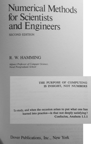
Quoting Hamming
During the discussion of the midterm exam, I repeated Hamming's aphorism that "the purpose of computing is insight, not numbers". Here's a photo of the cover page of Hamming's book, with an inset of his pithy comment from the page following the cover. The frontmatter also has another nice idea attributed to Confucius.
10. fzero wrap-up, Review for midterm, begin review of linear algebra
Lecture on 30 October 2008
Reading: pp. 273 - 279
9. Newton's method, Secant Method, fzero
Lecture on 28 October 2008
Reading: pp. 261 - 279
8. Bracketing and Bisection
Lecture on 23 October 2008
Reading: pp. 253 - 261
Learning Objectives
- Be able to describe the role of bracketing in the root-finding process
- Be able to describe the bisection algorithm for root-finding
- Be able to identify and write sample code for two different types of convergence criteria for a root-finding problem.
- Be able to use the
bisectroutine from the NMM Toolbox. - Be able to test whether the root-finding procedure produced a useful root.
Handouts
7. Introduction to root finding
Lecture on 21 October 2008
Reading: pp. 240 - 250, 253 - 261, skim pp. 250 - 253
Learning Objectives
- Be able to formulate a generic root-finding problem as f(x) = 0
- Be able to graphically locate the root of f(x) on a plot of f(x) versus x
- Be able to graphically locate brackets to roots of f(x)
- Be able to write an m-file function that computes f(x) in a way that is compatible with root-finding routines.
- Be able to describe the bisection algorithm for root-finding
6. Practical implications of floating point arithmetic
Lecture on 16 October 2008
Reading: pp. 193 - 197, 199 - 200, 209 - 213
The first half of the class was Quiz 1
This blog post by bre pettis shows you how to use your fingers to count in base two:
5. fprintf, Introduction to floating point arithmetic
Lecture on 14 October 2008
Reading: pp. 48 - 51, 101 - 105
Learning Objectives
- Be able to name the three MATLAB data types most commonly used in ME 352.
- Be able to use the
fprintfstatement to print strings and values stored in MATLAB variables..
codes
- demofprintf.m
- printFormat1.m
- printFormat2.m
- printFormat3.m
- printFormat4.m
- printFormat5.m
- printFormat6.m
Lecture Notes
History of the ASME
After Joel Rogers gave his presentation about the ASME HPV competition, I described the role of the ASME and the development of the Boiler Code. I got the facts wrong.
The ASME held its first meeting in November 1880. The Boiler code was published in 1914.
Refer to this page on the ASME web site for a Brief History of the ASME.
4. Conditional execution
Lecture on 9 October 2008
Reading: pp. 105 - 127
Learning Objectives
- Be able to give numerical values equivalent to the logical expressions "true" and "false".
- Be able to implement a basic "if ... else" construct
- Be able to read and modify a simple m-file for evaluating the series approximation to sin(x) with automatic truncation of the series.
codes
Handouts
3. MATLAB functions, Loops
Lecture on 7 October 2008
Reading: pp. 63-68, 85-86, 93-98
Learning Objectives
- Be able to describe the sequential execution of an m-file and how that is different from the calculations in a spreadsheet.
- Be able to implement a basic "for" loop
- Be able to write a m-file function to compute the factorial of n, where n is an integer.
- Be able to define "recursive" when it refers to evaluating terms in the sine series.
- Be able to read and modify a simple m-file for evaluating an n-term approximation to sin(x)
Handouts
2. MATLAB functions, input and output parameters
Lecture on 2 October 2008
Reading: pp. 63-68, 85-86, 93-98
Learning Objectives
- Be able to write simple MATLAB functions
- Be able to write a one-line MATLAB function to evaluate the three-term approximation to sin(x)
- Be able to write a short MATLAB function to plot discrete data and data generated from a formula.
Podcast Failure
The podcast of the lecture did not work. The record/pause buttons can sometimes be pressed accidentally when I put the recorder in my pocket. I suspect that happened.
CADLAB Work
The second half of the class was spent in the CADLAB (EB 325) working on some problems that should help prepare you to do the homework.
Handouts
1. Introduction, Motivation for Programing, MATLAB functions
Lecture on 29 September 2008
Reading: pp. 15-25, 63-68, 85-86, 93-98
Podcast: [Part A] [Part B] [Part C]
Learning Objectives
- Know how to contact GWR: email, telephone, office hours
- Be able find relevant information: handouts, textbook, website
- Be able to explain how this course fits into the curriculum.
- Be able to launch MATLAB
- Know how to assign variables and do basic calculations
- Be able to make a simple plot of y versus x
- Be able to write a simple function with one input variable and one output variable
Activate Your MCECS Account
All students will need to use MATLAB to complete the first problem set. You do not need to buy MATLAB because it is available on all the computers on the College network. To use those computers you must first activate your MCECS computer account by following these steps:
- Go to Room 60-06 in the Fourth Avenue Building
- Ask to have your account activated
- Follow directions given to you by the help desk worker in FAB 60-06
Refer to the New User Support Page for additional information.
Also consult the Schedule for the help desk
Textbook Reading
Chapter 1 provides an overview to numerical analysis and the structure of the book. This is useful background information. It would be helpful to reread this chapter about midway through the quarter when the vocabulary will have more meaning.
Chapter 2 describes how to use MATLAB to perform interactive calculations. Plotting is also covered in Chapter 2.
Chapter 3 describes how to write MATLAB programs. In this first lecture we only considered the task of encapsulating a few MATLAB statements in an m-file. In the next class we'll examine input and output parameters in more detail.
Prepare for Lecture 2
Students are expected to have completed the following tasks in preparation of class meeting #2:
- Activate your MCECS account
- Read assigned sections from the textbook
- Read the review notes on infinite series, and bring any questions to the next class meeting